空气流体中速度矢量场,噪声检测方案

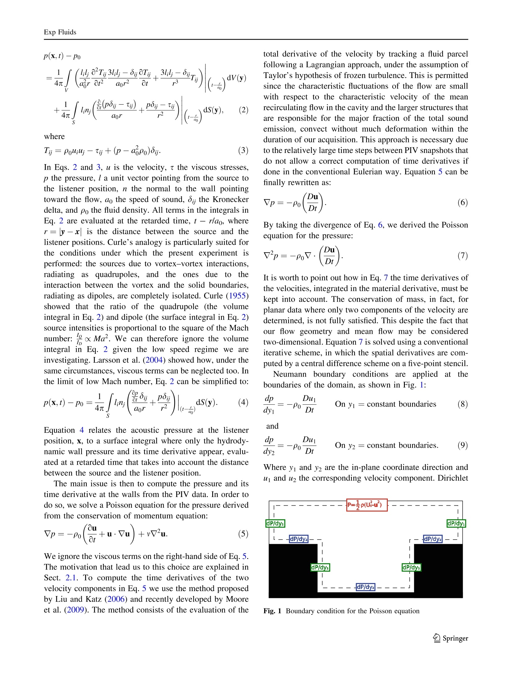
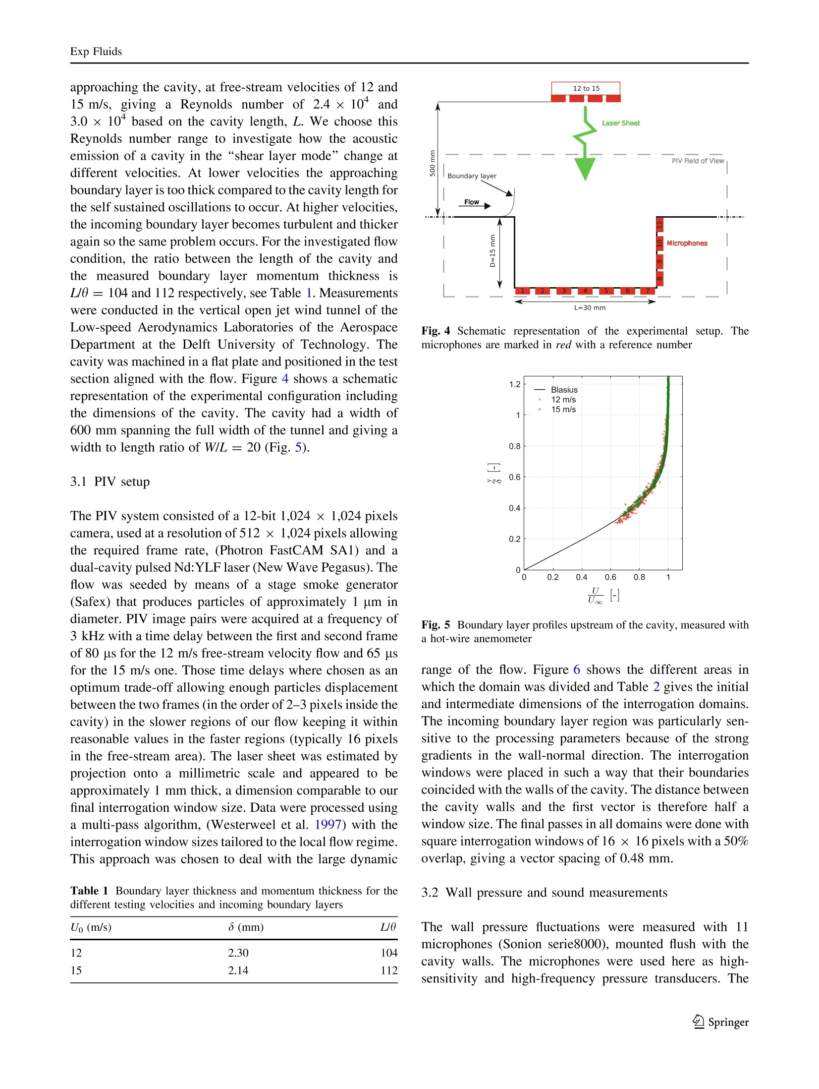
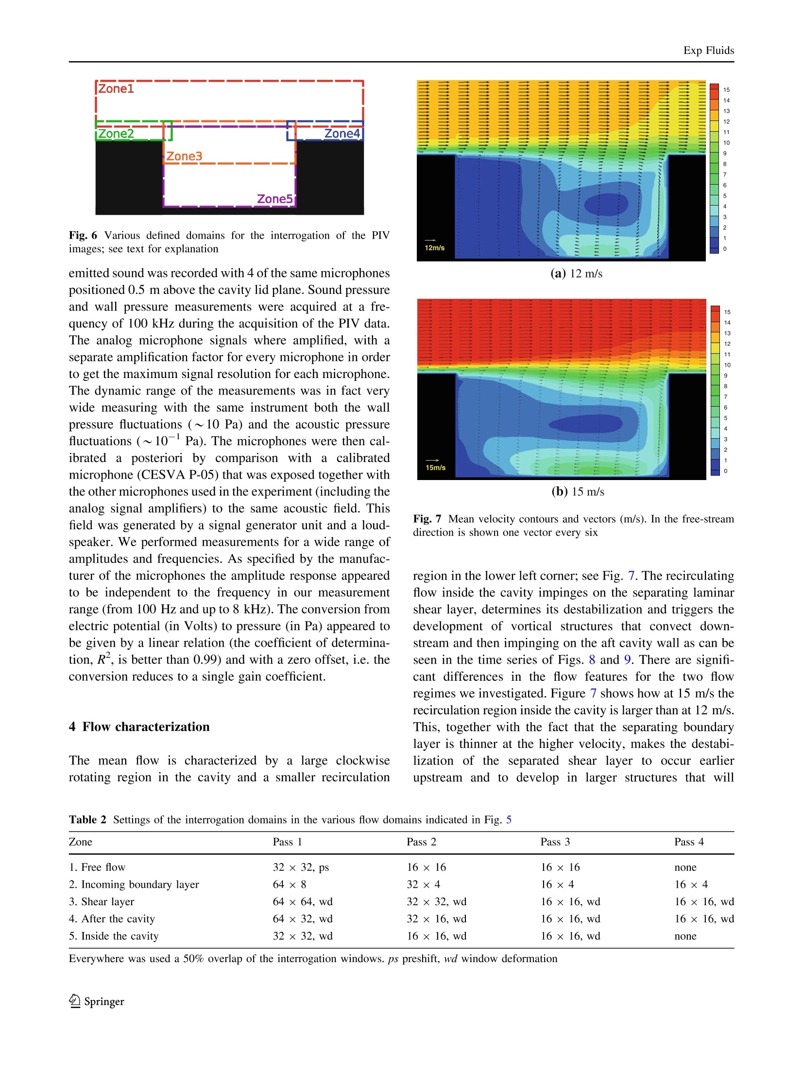
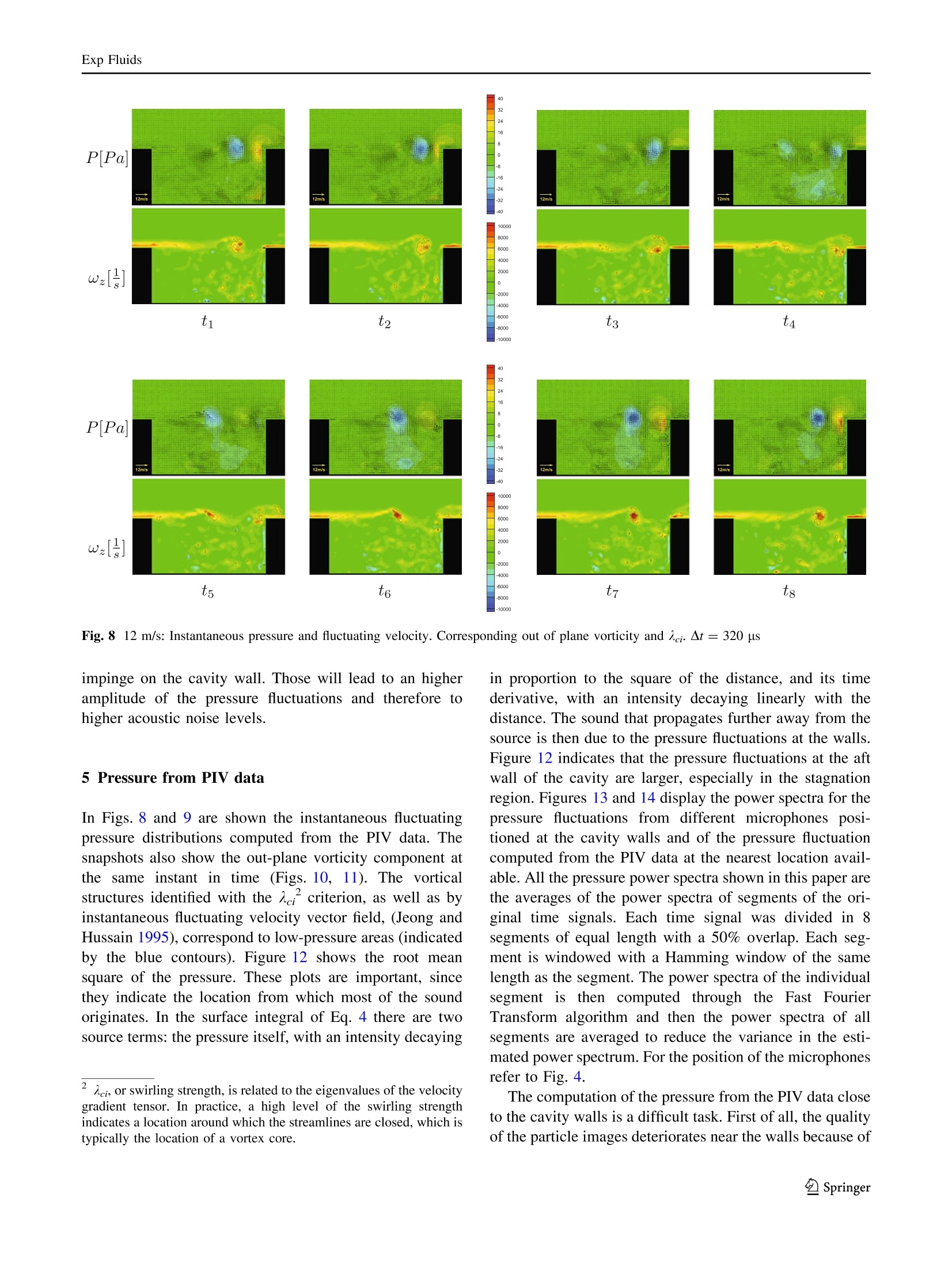
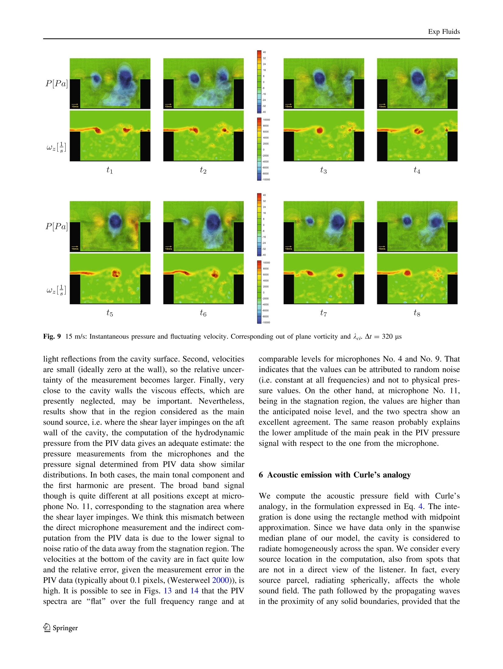
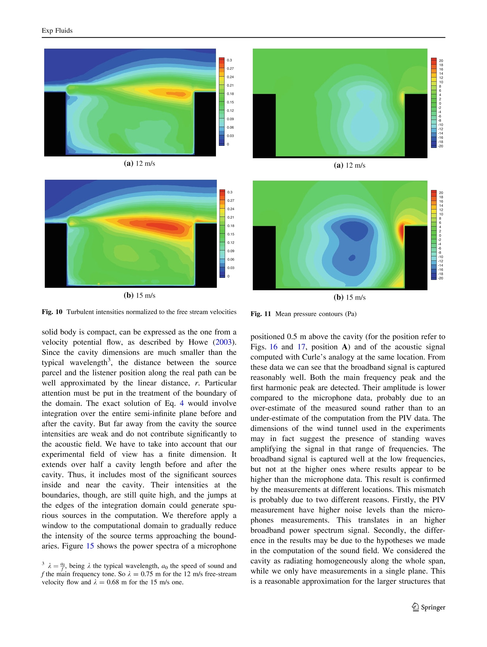
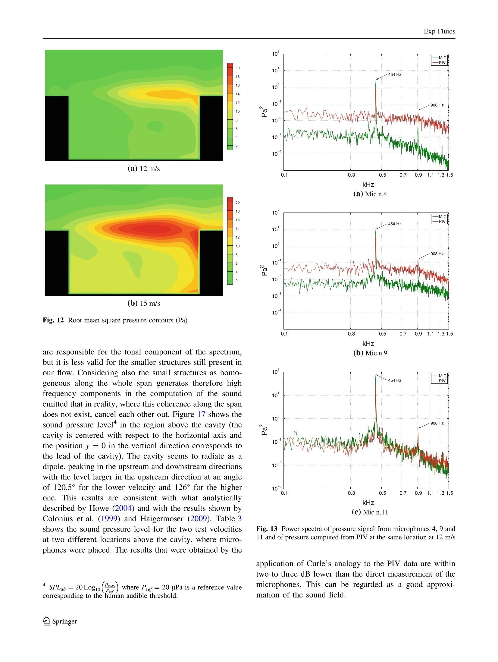
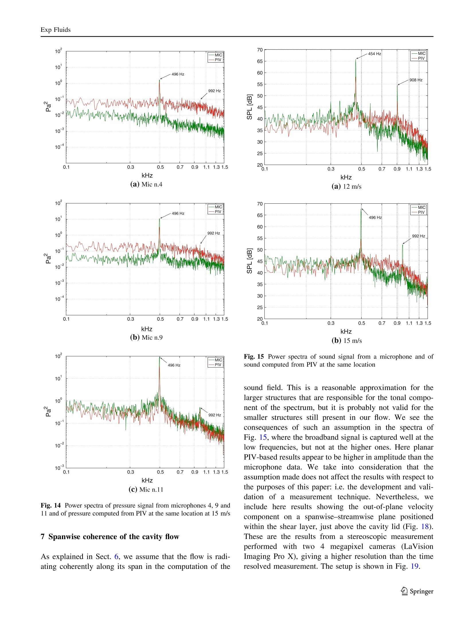
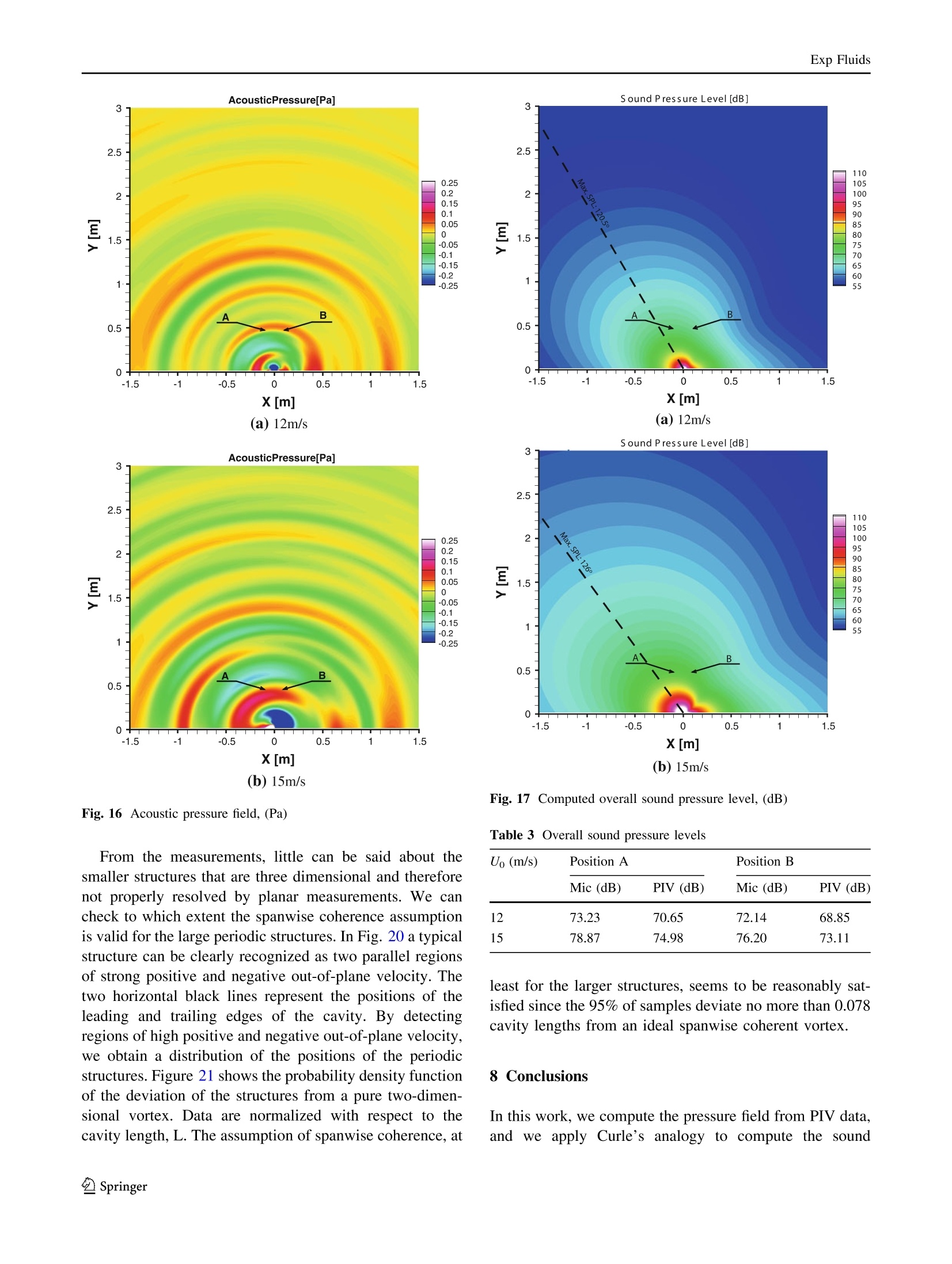
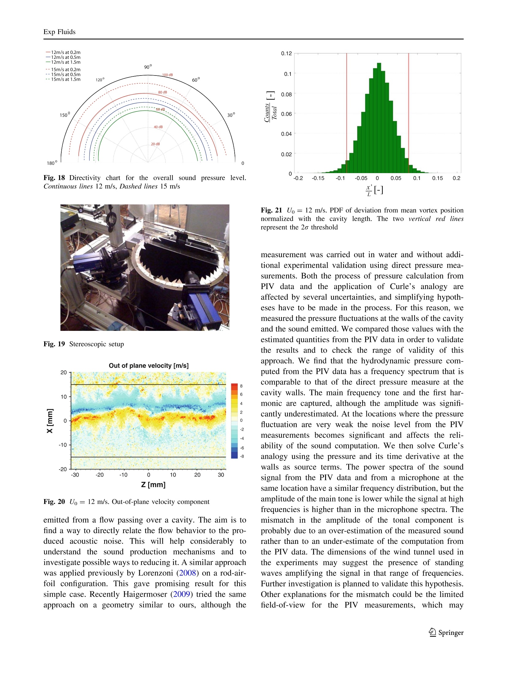
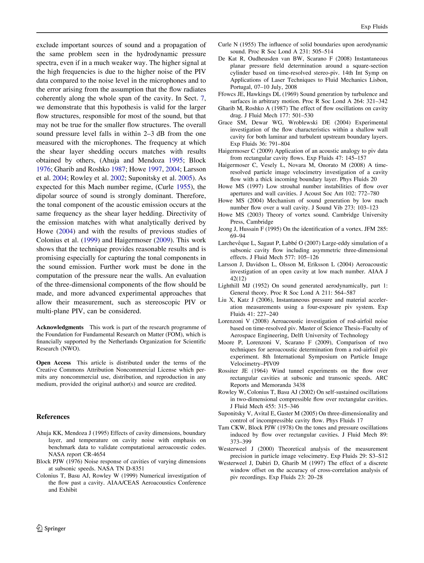
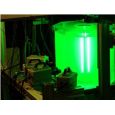
DOI 10.1007/s00348-010-0935-8 Exp Fluids High speed PIV applied to aerodynamic noise investigation . V. Koschatzky· P. D. Moore·J. Westerweel · F. Scarano·B. J. Boersma Received： 11 December 2009/Revised： 26 April 2010/Accepted： 2 July 2010 Abstract In this paper， we study the acoustic emissionsof the flow over a rectangular cavity. Especially， weinvestigate theepossibility of estimatingg itheacousticemission by analysis of PIV data. Such a possibility isappealing， since it would allow to directly relate the flowbehavior to the aerodynamic noise production. This willhelp considerably in understanding the noise productionmechanisms and to investigate the possible ways ofreducing it. In this study， we consider an open cavity withan aspect ratio between its length and depth of 2 at aReynolds number of 2.4 x 10 and 3.0 ×10 based on thecavity length. The study is carried out combining highspeed two-dimensional PIV， wall pressure measurementsand sound measurements. The pressure field is computedfrom the PIV data. Curle’s analogy is applied to obtain theacoustic pressure field. The pressure measurements on thewall of the cavity and the sound measurements are thenused to validate the results obtained from PIV and checkthe range of validity of this approach. This study demon-strated that the technique is able to quantify the acousticemissions from the cavity and is promising especially forcapturing the tonal components on the sound emission. V. Koschatzky (区)·J. Westerweel· B. J. BoersmaLaboratory for Aero and Hydrodynamics，Faculty of Mechanical， Maritime and Materials Engineering，Delft University of Technology， Delft， The Netherlandse-mail： v.koschatzky@tudelft.nl P. D. Moore · F. Scarano ( High Speed L a boratory， Faculty of Aerospace En g ineeringDelft U niversity o f T echnology， Delft， The Netherlands ) l Introduction The generation of noise by flow over a rectangular cavityis an important benchmark problem for aeroacoustics andhas been investigated both experimentally and numericallyin the last decades (Rowley et al. 2002). Because of therelevance for aeronautic applications most of the researchhas been done on flows at a high Mach number， wherecompressibility effects are important. Much less attentionhas been put in low Mach number cavity flows， typical ofdifferent ground and submarine applications. Therefore，this work focuses on cavity flows at low Mach numbers toinvestigate the possibility of estimating theie acousticemission by analysis of PIV data. Ahuja and Mendoza(1995) have shown how the flow that generates pastcavities depends on multiple factors such as the cavitygeometry， the free stream velocity and the incomingboundary layer properties. Gharib and Roshko (1987)identified different flows behaviors arising in flows overrectangular open cavities. They showed that， when theratio between the cavity length and the boundary layermomentum thicknessisislarger than a certain value(L/0> 80-100 depending on other parameters) theshear layer separating at the leading edge of the cavitydevelops in large scale coherent spanwise vortices. Theynamed this flow regime “shear layer mode” At highervalues of L/0 (>120) the “wake mode” occurs. In the“wake mode" the structures become comparable to thecavity dimensions. The external flow alternatively entersinto the cavity reattaching to the bottom and ejects out ofit. The “wake mode" has been rarely observed in exper-iments， while it occurs often in numerical simulations ( A cavity is called open when the ratio between its length and depth i s larger than one. ) where three-dimensional perturbations of the incomingflow can be completely avoided and periodic boundaryconditionss arare a commonpractice in thee transversedirection， (Larcheveque et al.22007； Suponitsky et al.2005). In the “shear layer mode”the vortical structuresperiodically impinge on the aft wall of the cavity， pro-ducing pressure fluctuations that radiate acoustic wavesand generate a self-sustaining oscillation mechanism. Thismechanism has a double nature： acoustic and hydrody-namic. Which one willpredominate depends on thewavelength of the perturbation and therefore on the flowspeed and the characteristic dimension of the cavity， thelength. In low-speed flows， the cavity can be considered asacoustically compact： its length is much smaller than theacoustic wavelength. Therefore， the acoustic perturbationis not able to influence the flow behavior in the cavity andtheeself-sustaininggoscillationmechanism is purelyhydrodynamic. It consists of a recirculating vortex insidethe cavity that impinges on the shear layer enhancing andtriggering its destabilization. Rossiter (1964) proposed anempirical formula to predict the frequencies of the cavityresonant modes： Here， St is the Strouhal number， fis the frequency， L thelength of the cavity， Uo the free stream velocity， Ma theMachi number， k the ratio between the shear layerconvection velocity and the free stream velocity， m themode number and y an empirical constant set to 0.25. TheRossiter equation gives accurate predictions， but failsat very low Mach numbers (Ma <0.2)， (Howe 1997). Thecomplexity of the flow and its strong time dependencehas made investigations difficult and not completelyexhaustive. Numerical simulations are limited by theavailable computational power. While numerical studiesare have been performed， at higher Reynolds numbers(increasing turbulence levels) and for complex geometries(such as cavities)， due to resolution requirements， modelingof the constitutive equations becomes necessary leadingoften to results in disaccord with the experimentalexperience， showing for example a higher occurrence ofthe“wake mode”(Colonius et al. 1999；Suponitsky et al.2005). Also few experiments have managed to obtainsatisfactory simultaneous measurements of both spatial andtemporal variations in a cavity. They have usually beenconfined to single-point time-resolved measurements orfull-field PIV imaging at low speeds， (Ahuja and Mendoza1995； Block 1976； Grace et al. 2004； Tam and Block1978). Some more recent attempts， such as that ofHaigermoser et al. (2008) and Haigermoser (2009)， haveperformed time-resolved PIV measurements， ini waterflows and at low free-stream velocity. A noticeable step forward but at conditions that are not yet representative ofsignificant acoustic noise generation. Recent developmentsin laser and camera technology allow the possibility toextend PIV to the study of aeroacoustic phenomena in airflows at moderate speed (up to V =20 m/s， Ma= 0.08).The aim of the present study is to make use of these newpossibilities， and to obtain estimates of the acousticemission from time-resolved PIV data. In order to do thatwe split the problem in two parts： we first compute thehydrodynamic pressure from the PIV velocity fields usingthe Navier-Stokes equations. The approach we followed isthe one proposed by Liu and Katz (2006) and De Kat et a.(2008) further developed by Moore et al. (2009). We thenapply Curle’s acoustic analogy， in the form suggested byLarsson et al. (2004)， to obtain the acoustic pressure field.However， it is well known that aeroacoustic predictionscan be sensitive to both measurement and numericaluncertainties. Therefore we test the robustness of ourmethod by comparing the results for the pressure and forthe acoustic pressure obtained from PIVwith directmeasurements of the pressure on the cavity walls and ofthe emitted sound， by means of several transducers. Thisapproach is only valid in the case of a compact cavity，where the feedback loop triggering the flow instability， thatis the source of sound， can be considered as purelyhydrodynamic. Therefore， the flow behavior and theacoustic emission are not coupled. 2 Acoustic pressure prediction from PIV data It is worth emphasizing that by using PIV we do notattempt to resolve acoustic fluctuations directly. Usuallyresearchers are interested in acoustic levels at a certaindistance from the source. This means that a relevantacoustic field is commonly much larger than the sourcefield. But imaging large areas reduces the spatial resolutionof the measurements. Furthermore， the magnitude of theacoustic pressure fluctuations isis orders of magnitudesmaller than the hydrodynamic pressure fluctuations andcertainly cannot be resolved within the measurement cer-tainty. Therefore， it is necessary to model the problem，linking the acoustic emission to quantities that can bemeasured reliably. Acoustic analogies have been derivedthat relate the acoustic pressure to flow quantities that areeasily obtained from measurements or computation such ashydrodynamic pressure or vorticity (Curle 1955； Ffowesand Hawkings 1969； Howe 2004，2003； Lighthill 1952).Those models are obtained under specific assumptions andmust be carefully chosen depending on the specific situa-tion. In the present study we apply Curle’s analogy， in theform derived by Larsson et al. (2004)， to compute acousticpressure from the PIV data： p(x，t)-po where In Eqs. 2 and 3， u is the velocity， t the viscous stresses， p the pressure， I a unit vector pointing from the source tothe listener position， n the normal to the wall pointingtoward the flow， ao the speed of sound， 8， the Kroneckerdelta， and po the fluid density. All terms in the integrals inEq. 2 are evaluated at the retarded time， t-rlao， wherer= y-x is the distance between the source and thelistener positions. Curle’s analogy is particularly suited forthe conditions under which the present experiment isperformed： the sources due to vortex-vortex interactions，radiating as gquadrupoles， and the onesdue to theinteraction between the vortex and the solid boundaries，radiating as dipoles， are completely isolated. Curle (1955)showed that the ratio of the quadrupole (the volumeintegral in Eq. 2) and dipole (the surface integral in Eq. 2)source intensities is proportional to the square of the Machnumber：o MaI’. We can therefore ignore the volumeintegral in Eq. 2 given the low speed regime we areinvestigating. Larsson et al. (2004) showed how， under thesame circumstances， viscous terms can be neglected too. Inthe limit of low Mach number， Eq. 2 can be simplified to： Equation 4 relates the acoustic pressure at the listenerposition， x， to a surface integral where only the hydrody-namic wall pressure and its time derivative appear， evalu-ated at a retarded time that takes into account the distancebetween the source and the listener position. The main issue is then to compute the pressure and itstime derivative at the walls from the PIV data. In order todo so， we solve a Poisson equation for the pressure derivedfrom the conservation of momentum equation： We ignore the viscous terms on the right-hand side of Eq. 5.The motivation that lead us to this choice are explained inSect. 2.1. To compute the time derivatives of the twovelocity components in Eq. 5 we use the method proposedby Liu and Katz (2006) and recently developed by Mooreet al. (2009). The method consists of the evaluation of the total derivative of the velocity by tracking a fluid parcelfollowing a Lagrangian approach， under the assumption ofTaylor’s hypothesis of frozen turbulence. This is permittedsince the characteristic fluctuations of the flow are smallwith respect to the characteristic velocity of the meanrecirculating flow in the cavity and the larger structures thatare responsible for the major fraction of the total soundemission， convect without much deformation within theduration of our acquisition. This approach is necessary dueto the relatively large time steps between PIV snapshots thatdo not allow a correct computation of time derivatives ifdone in the conventional Eulerian way. Equation 5 can befinally rewritten as： By taking the divergence of Eq. 6， we derived the Poissonequation for the pressure： It is worth to point out how in Eq. 7 the time derivatives ofthe velocities， integrated in the material derivative， must bekept into account. The conservation of mass， in fact， forplanar data where only two components of the velocity aredetermined， is not fully satisfied. This despite the fact thatour flow geometry and mean flow may be consideredtwo-dimensional. Equation 7 is solved using a conventionaliterative scheme， in which the spatial derivatives are com-puted by a central difference scheme on a five-point stencil. Neumanntboundary conditionsareapplieddat ttheboundaries of the domain， as shown in Fig. 1： Where yi and y2 are the in-plane coordinate direction andu and u2 the corresponding velocity component. Dirichlet Fig. 1 Boundary condition for the Poisson equation boundary conditions are applied at the upper limit of thedomain： 2.1 On the viscous terms We follow the approach suggested by Liu and Katz (2006)).In their paper they point out that in a high Reynolds numberflow field located away from boundaries， the materialacceleration is dominant and the viscous term is negligibleAdditionally their results confirmed that， for cases comparable to our own， the material acceleration is the dominantterm in Eq. 5 and the other terms can be neglected. Theyalso note that one should be careful in evaluating the con-tribution of the viscous term and avoid integrating alongpaths that are particularly affected by viscosity，e.g.， along aboundary layer.With our set of equations we can say thefollowing： ignoring viscous terms in Eq. 5 only affects theNeumann boundary conditions (8) and (9). The Poisson Eq.7 would be without the viscous terms anyway， because ofthe mass conservation. Due to the relatively high Reynoldsnumbers we are considering in this study， the viscouseffects are significant only in a small region close to thewall. The computation of the pressure does not need to becarried out fully to the present walls. We then apply theboundary conditions not directly at the walls but 2 vectorsrows (corresponding to a distance of 0.96 mm) away fromthem. A distance considered sufficient to be surely out ofthe viscous layer， but close enough to estimate correctly thepressure at the walls (the pressure does not vary signifi-cantly in the direction normal to the wall). Moreover， thecomputation of those terms involves a double spatial dif-ferentiation of the velocity data field， an operation thatstrongly amplifies signal noise which will lead to a domi-nating contribution to the final result. Figure 2 shows themean of the pressure gradient of Eq. 5， the contribution ofthe acceleration term and the contribution of the viscousterm magnified 100 times (Fig. 3). It is clear that the viscousterm has high values close to the walls. But its magnitude isaround two orders of magnitude lower than the accelerationterm. As a result， the total pressure gradient is not sub-stantially affected by ignoring the viscous term. The resultsin Sect. 5 also confirm the validity of our assumption 3 Experimental setup The study was carried out combining high-speed planar PIVimaging， wall pressure measurements， and sound measurements. The boundary layer was also measured at theleading edge of the cavity with a hot wire anemometer. Weperformed experiments with a laminar boundary layer flow (a) Pressure gradient [] (b) Acceleration term[] Fig. 2 Mean pressure gradient at 12 m/s. Total， acceleration termand viscous term. One vector every two is displayed approaching the cavity， at free-stream velocities of 12 and15 m/s， giving a Reynolds number of 2.4×104 and3.0 ×10 based on the cavity length， L. We choose thisReynolds number range to investigate how the acousticemission of a cavity in the “shear layer mode” change atdifferent velocities. At lower velocities the approachingboundary layer is too thick compared to the cavity length forthe self sustained oscillations to occur. At higher velocities，the incoming boundary layer becomes turbulent and thickeragain so the same problem occurs. For the investigated flowcondition， the ratio between the length of the cavity andthe measured boundary layer momentum thickness isL/0 = 104 and 112 respectively， see Table 1.Measurementswere conducted in the vertical open jet wind tunnel of theLow-speed Aerodynamics Laboratories of the AerospaceDepartment at the Delft University of Technology. Thecavity was machined in a flat plate and positioned in the testsection aligned with the flow. Figure 4 shows a schematicrepresentation of the experimental configuration includingthe dimensions of the cavity. The cavity had a width of600 mm spanning the full width of the tunnel and giving awidth to length ratio of W/L =20 (Fig.5). 3.1 PIV setup The PIV system consisted ofa 12-bit 1，024× 1，024 pixelscamera， used at a resolution of 512×1，024 pixels allowingthe required frame rate， (Photron FastCAM SA1) and adual-cavity pulsed Nd：YLF laser (New Wave Pegasus). Theflow was seeded by means of a stage smoke generator(Safex) that produces particles of approximately 1 um indiameter. PIV image pairs were acquired at a frequency of3 kHz with a time delay between the first and second frameof 80 us for the 12 m/s free-stream velocity flow and 65 usfor the 15 m/s one. Those time delays where chosen as anoptimum trade-off allowing enough particles displacementbetween the two frames (in the order of 2-3 pixels inside thecavity) in the slower regions of our flow keeping it withinreasonable values in the faster regions (typically 16 pixelsin the free-stream area). The laser sheet was estimated byprojection onto a millimetric scale and appeared to beapproximately 1 mm thick， a dimension comparable to ourfinal interrogation window size. Data were processed usinga multi-pass algorithm， (Westerweel et al. 1997) with theinterrogation window sizes tailored to the local flow regime.This approach was chosen to deal with the large dynamic Table 1 Boundary layer thickness and momentum thickness for thedifferent testing velocities and incoming boundary layers Uo (m/s) o(mm) L/0 12 2.30 104 15 2.14 112 Fig. 4 Schematic representation of the experimental setup. Themicrophones are marked in red with a reference number Fig. 5 Boundary layer profiles upstream of the cavity， measured witha hot-wire anemometer range of the flow. Figure 6 shows the different areas inwhich the domain was divided and Table 2 gives the initialand intermediate dimensions of the interrogation domains.The incoming boundary layer region was particularly sen-sitive to the processing parameters because of the stronggradients in the wall-normal direction. The interrogationwindows were placed in such a way that their boundariescoincided with the walls of the cavity. The distance betweenthe cavity walls and the first vector is therefore half awindow size. The final passes in all domains were done withsquare interrogation windows of 16 × 16 pixels with a 50%overlap， giving a vector spacing of 0.48 mm. 3.2 Wall pressure and sound measurements The wall pressure fluctuationsis were measured with 11microphones (Sonion serie8000)， mounted flush with thecavity walls. The microphones were used here as high-sensitivity and high-frequency pressure transducers. The Fig. 6 Various defined domains for the interrogation of the PIVimages； see text for explanation emitted sound was recorded with 4 of the same microphonespositioned 0.5 m above the cavity lid plane. Sound pressureand wall pressure measurements were acquired at a fre-quency of 100 kHz during the acquisition of the PIV dataThe analog microphone signals where amplified， with aseparate amplification factor for every microphone in orderto get the maximum signal resolution for each microphone.The dynamic range of the measurements was in fact verywide measuring with the same instrument both the wallpressure fluctuations (~10Pa) and the acoustic pressurefluctuations (~10- Pa). The microphones were then cal-ibrated a posteriori by comparison with a calibratedmicrophone (CESVA P-05) that was exposed together withthe other microphones used in the experiment (including theanalog signal amplifiers) to the same acoustic field. Thisfield was generated by a signal generator unit and a loud-speaker. We performed measurements for a wide range ofamplitudes and frequencies. As specified by the manufac-turer of the microphones the amplitude response appearedto be independent to the frequency in our measurementrange (from 100 Hz and up to 8 kHz). The conversion fromelectric potential (in Volts) to pressure (in Pa) appeared tobe given by a linear relation (the coefficient of determina-tion， R’， is better than 0.99) and with a zero offset， i.e. theconversion reduces to a single gain coefficient. 4 Flow characterization The mean flow is characterized by a large clockwiserotating region in the cavity and a smaller recirculation (a) 12 m/s (b) 15 m/s Fig. 7 Mean velocity contours and vectors (m/s). In the free-streamdirection is shown one vector every six region in the lower left corner； see Fig. 7. The recirculatingflow inside the cavity impinges on the separating laminarshear layer， determines its destabilization and triggers thedevelopment of vortical structures that convect down-stream and then impinging on the aft cavity wall as can beseen in the time series of Figs. 8 and 9. There are signifi-cant differences in the flow features for the two flowregimes we investigated. Figure 7 shows how at 15 m/s therecirculation region inside the cavity is larger than at 12 m/s.This， together with the fact that the separating boundarylayer is thinner at the higher velocity， makes the destabi-lization of the separated shear layer to occur earlierupstream and to develop in larger structures that will Table 2 Settings of the interrogation domains in the various flow domains indicated in Fig. 5 Zone Pass 1 Pass 2 Pass 3 Pass 4 1. Free flow 32 × 32， ps 16 x16 16×16 none 2. Incoming boundary layer 64×8 32x4 16 x4 16×4 3. Shear layer 64 x 64， wd 32 × 32， wd 16 ×16， wd 16 × 16， wd 4. After the cavity 64×32， wd 32 ×16， wd 16 x16， wd 16 × 16， wd 5. Inside the cavity 32 x 32， wd 16 × 16， wd 16 × 16， wd none 40 Fig. 8 12 m/s： Instantaneous pressure and fluctuating velocity. Corresponding out of plane vorticity and Aci. At=320 us impinge on the cavity wall. Those will lead to an higheramplitude of the pressure fluctuations and therefore tohigher acoustic noise levels. 5 Pressure from PIV data In Figs. 8 and 9 are shown the instantaneous fluctuatingpressure distributions computed from the PIV data. Thesnapshots also show the out-plane vorticity component atthe same instant in time (Figs. 10， 11). The vorticalstructures identified with the acriterion， as well as byinstantaneous fluctuating velocity vector field， (Jeong andHussain 1995)， correspond to low-pressure areas (indicatedby the blue contours). Figure 12 shows the root meansquare of the pressure. These plots are important， sincethey indicate the location from which most of the soundoriginates. In the surface integral of Eq. 4 there are twosource terms： the pressure itself， with an intensity decaying ( Ac i ， or swirling strength， i s related to t he eigenvalues of the velocitygradient t ensor. I n practice， a h i gh le v el of th e sw i rling str e ngth indicates a location around which the streamlines a re closed， which i s typically t he l ocation o f a v ortex core. ) in proportion to the square of the distance， and its timederivative， with an intensity decaying linearly with thedistance. The sound that propagates further away from thesource is then due to the pressure fluctuations at the walls.Figure 12 indicates that the pressure fluctuations at the aftwall of the cavity are larger， especially in the stagnationregion. Figures 13 and 14 display the power spectra for thepressure fluctuations from different microphones posi-tioned at the cavity walls and of the pressure fluctuationcomputed from the PIV data at the nearest location avail-able. All the pressure power spectra shown in this paper arethe averages of the power spectra of segments of the ori-ginal time signals. Each time signal was divided in 8segments of equal length with a 50% overlap. Each seg-ment is windowed with a Hamming window of the samelength as the segment. The power spectra of the individualsegment is then computed through the Fast FourierTransform algorithm and then the power spectra of allsegments are averaged to reduce the variance in the esti-mated power spectrum. For the position of the microphonesrefer to Fig. 4. The computation of the pressure from the PIV data closeto the cavity walls is a difficult task. First of all， the qualityof the particle images deteriorates near the walls because of 40 Fig. 9 15 m/s： Instantaneous pressure and fluctuating velocity. Corresponding out of plane vorticity and Aci. At= 320 us light reflections from the cavity surface. Second， velocitiesare small (ideally zero at the wall)， so the relative uncer-tainty of the measurement becomes larger. Finally， veryclose to the cavity walls the viscous effects， which arepresently neglected， may be important. Nevertheless，results show that in the region considered as the mainsound source， i.e. where the shear layer impinges on the aftwall of the cavity， thecomputation of the hydrodynamicpressure from the PIV data gives an adequate estimate： thepressure measurements from the microphones and thepressure signal determined from PIV data show similardistributions. In both cases， the main tonal component andthe first harmonic are present. The broad band signalthough is quite different at all positions except at micro-phone No. 11， corresponding to the stagnation area wherethe shear layer impinges. We think this mismatch betweenthe direct microphone measurement and the indirect com-putation from the PIV data is due to the lower signal tonoise ratio of the data away from the stagnation region. Thevelocities at the bottom of the cavity are in fact quite lowand the relative error， given the measurement error in thePIV data (typically about 0.1 pixels，(Westerweel 2000))， ishigh. It is possible to see in Figs. 13 and 14 that the PIVspectra are “flat" over the full frequency range and at comparable levels for microphones No. 4 and No. 9. Thatindicates that the values can be attributed to random noise(i.e. constant at all frequencies) and not to physical pres-sure values. On the other hand， at microphone No. 11，being in the stagnation region， the values are higher thanthe anticipated noise level， and the two spectra show anexcellent agreement. The same reason probably explainsthe lower amplitude of the main peak in the PIV pressuresignal with respect to the one from the microphone. 6 Acoustic emission with Curle’s analogy We compute the acoustic pressure field with Curle’sanalogy， in the formulation expressed in Eq. 4. The inte-gration is done using the rectangle method with midpointapproximation. Since we have data only in the spanwisemedian plane of our model， the cavity is considered toradiate homogeneously across the span. We consider everysource location in the computation， also from spots thatare not in a direct view of the listener. In fact， everysource parcel， radiating spherically， affects the wholesound field. The path followed by the propagating wavesin the proximity of any solid boundaries， provided that the (a) 12 m/s (a) 12 m/s (b) 15 m/s (b) 15 m/s Fig. 10 Turbulent intensities normalized to the free stream velocities solid body is compact， can be expressed as the one from avelocity potential flow， as described by Howe (2003).Since the cavity dimensions are much smaller than thetypical wavelength， the distance between the sourceparcel and the listener position along the real path can bewell approximated by the linear distance， r. Particularattention must be put in the treatment of the boundary ofthe domain. The exact solution of Eq. 4 would involveintegration over the entire semi-infinite plane before andafter the cavity. But far away from the cavity the sourceintensities are weak and do not contribute significantly tothe acoustic field. We have to take into account that ourexperimental field of view has a finite dimension. Itextends over half a cavity length before and after thecavity. Thus， it includes most of the significant sourcesinside and near the cavity. Their intensities attheboundaries， though， are still quite high， and the jumps atthe edges of the integration domain could generate spu-rious sources in the computation. We therefore apply awindow to the computational domain to gradually reducethe intensity of the source terms approaching the bound-aries. Figure 15 shows the power spectra of a microphone ( ’ A = 4o， be i ng a the typical wavelength， ao the sp e ed of sound and f the main f r equency tone. So 1 = 0.75 m for the 12 m/s free-stream velocity flow and a=0.68 m for the 15 m/s one. ) Fig. 11 Mean pressure contours (Pa) positioned 0.5 m above the cavity (for the position refer toFigs. 16 and 17， position A) and of the acoustic signalcomputed with Curle’s analogy at the same location. Fromthese data we can see that the broadband signal is capturedreasonably well. Both the main frequency peak and thefirst harmonic peak are detected. Their amplitude is lowercompared to the microphone data， probably due to anover-estimate of the measured sound rather than to anunder-estimate of the computation from the PIV data. Thedimensions of the wind tunnel used in the experimentsmay in fact suggest the presence of standing wavesamplifying the signal in that range of frequencies. Thebroadband signal is captured well at the low frequencies，but not at the higher ones where results appear to behigher than the microphone data. This result is confirmedby the measurements at different locations. This mismatchis probably due to two different reasons. Firstly， the PIVmeasurement have higher noise levels than the micro-phonessmeasurements.Thisisttranslatesin an higherbroadband power spectrum signal. Secondly， the differ-ence in the results may be due to the hypotheses we madein the computation of the sound field. We considered thecavity as radiating homogeneously along the whole span，while we only have measurements in a single plane. Thisis a reasonable approximation for the larger structures that (a) 12 m/s Fig. 12 Root mean square pressure contours (Pa) are responsible for the tonal component of the spectrum，but it is less valid for the smaller structures still present inour flow. Considering also the small structures as homo-geneous along the whole span generates therefore highfrequency components in the computation of the soundemitted that in reality， where this coherence along the spandoes not exist， cancel each other out. Figure 17 shows thesound pressure level in the region above the cavity (thecavity is centered with respect to the horizontal axis andthe position y=0 in the vertical direction corresponds tothe lead of the cavity). The cavity seems to radiate as adipole， peaking in the upstream and downstream directionswith the level larger in the upstream direction at an angleof 120.5° for the lower velocity and 126° for the higherone. This results are consistent with what analyticallydescribed by Howe (2004) and with the results shown byColonius et al. (1999) and Haigermoser (2009). Table 3shows the sound pressure level for the two test velocitiesat two different locations above the cavity， where micro-phones were placed. The results that were obtained by the ( “ SPLdb = 20Lo P g10( RMS Pr w here P r ef= 20 p P a is a reference value e f corresponding to the human audible threshold. ) kHz (a) Mic n.4 (c) Mic n.11 Fig. 13 Power spectra of pressure signal from microphones 4，9 and11 and of pressure computed from PIV at the same location at 12 m/s application of Curle’s analogy to the PIV data are withintwo to three dB lower than the direct measurement of themicrophones. This can be regarded as a good approxi-mation of the sound field. 10* -MIC PIV 10 -496 Hz 10° 992 Hz 10 MA 10 咪h 103 Fig. 14 Power spectra of pressure signal from microphones 4， 9 and11 and of pressure computed from PIV at the same location at 15 m/s 7 Spanwise coherence of the cavity flow As explained in Sect. 6， we assume that the flow is radi-ating coherently along its span in the computation of the -454 Hz： -MIC-PIV 908 Hz (a) 12 m/s Fig. 15 Power spectra of sound signal from a microphone and ofsound computed from PIV at the same location sound field. This is a reasonable approximation for thelarger structures that are responsible for the tonal compo-nent of the spectrum， but it is probably not valid for thesmaller structures still present in our flow. We see theconsequences of such an assumption in the spectra ofFig. 15， where the broadband signal is captured well at thelow frequencies， but not at the higher ones. Here planarPIV-based results appear to be higher in amplitude than themicrophone data. We take into consideration that theassumption made does not affect the results with respect tothe purposes of this paper： i.e. the development and vali-dation of a measurement technique. Nevertheless， weinclude here results showing the out-of-plane velocitycomponent on a spanwise-streamwise plane positionedwithin the shear layer， just above the cavity lid (Fig. 18).These are the results from a stereoscopic measurementperformed with two 41 rmegapixel cameras (LaVisionImaging Pro X)， giving a higher resolution than the timeresolved measurement. The setup is shown in Fig. 19. S ound Pres s ure Level [dB] X[m] (a) 12m/s 3 2.5 110 105 2 100 E1.5 TT T T--1 -0.5 0 0.5X[m](a) 12m/sS ound P ressure Level [dB]\ 0.5 0 1 -1.5 -1 -0.5 0 0.5 1.5 X[m] (b) 15m/s (b) 15m/s Fig. 17 Computed overall sound pressure level， (dB) Fig. 16 Acoustic pressure field， (Pa) Table 3 Overall sound pressure levels From the measurements， little can be said about thesmaller structures that are three dimensional and thereforenot properly resolved by planar measurements. We cancheck to which extent the spanwise coherence assumptionis valid for the large periodic structures. In Fig. 20 a typicalstructure can be clearly recognized as two parallel regionsof strong positive and negative out-of-plane velocity. Thetwo horizontal black lines represent the positions of theleading and trailing edges of the cavity. By detectingregions of high positive and negative out-of-plane velocity，we obtain a distribution of the positions of the periodicstructures. Figure 21 shows the probability density functionof the deviation of the structures from a pure two-dimen-sional vortex. Data are normalized with respect to thecavity length， L. The assumption of spanwise coherence， at Uo (m/s) Position A Position B Mic (dB) PIV (dB) Mic (dB) PIV (dB) 12 73.23 70.65 72.14 68.85 15 78.87 74.98 76.20 73.11 least for the larger structures， seems to be reasonably sat-isfied since the 95% of samples deviate no more than 0.078cavity lengths from an ideal spanwise coherent vortex. 8 Conclusions In this work， we compute the pressure field from PIV data，and we apply Curle’s analogy to compute the sound 0 Fig. 18 Directivity chart for the overall sound pressure level.Continuous lines 12 m/s， Dashed lines 15 m/s Fig. 19 Stereoscopic setup Fig. 20 Uo= 12 m/s. Out-of-plane velocity component emitted from a flow passing over a cavity. The aim is tofind a way to directly relate the flow behavior to the pro-duced acoustic noise. This will help considerably tounderstand the sound production mechanisms and toinvestigate possible ways to reducing it. A similar approachwas applied previously by Lorenzoni (2008) on a rod-air-foil configuration. This gave promising result for thissimple case. Recently Haigermoser (2009) tried the sameapproach on a geometry similar to ours， although the Fig. 21 Uo= 12 m/s. PDF of deviation from mean vortex positionnormalized with the cavity length. The two vertical red linesrepresent the 2o threshold measurement was carried out in water and without addi-tional experimental validation using direct pressure mea-surements. Both the process of pressure calculation fromPIV data and the application of Curle’s analogy areaffected by several uncertainties， and simplifying hypoth-eses have to be made in the process. For this reason， wemeasured the pressure fluctuations at the walls of the cavityand the sound emitted. We compared those values with theestimated quantities from the PIV data in order to validatethe results and to check the range of validity of thisapproach. We find that the hydrodynamic pressure com-puted from the PIV data has a frequency spectrum that iscomparable to that of the direct pressure measure at thecavity walls. The main frequency tone and the first har-monic are captured， although the amplitude was signifi-cantly underestimated. At the locations where the pressurefluctuation are very weak the noise level from the PIVmeasurements becomes significant and affects the reli-ability of the sound computation. We then solve Curle’sanalogy using the pressure and its time derivative at thewalls as source terms. The power spectra of the soundsignal from the PIV data and from a microphone at thesame location have a similar frequency distribution， but theamplitude of the main tone is lower while the signal at highfrequencies is higher than in the microphone spectra. Themismatch in the amplitude of the tonal component isprobably due to an over-estimation of the measured soundrather than to an under-estimate of the computation fromthe PIV data. The dimensions of the wind tunnel used inthe experiments may suggest the presence of standingwaves amplifying the signal in that range of frequencies.Further investigation is planned to validate this hypothesis.Other explanations for the mismatch could be the limitedfield-of-view for the PIV mieasurements， whichmay exclude important sources of sound and a propagation ofthe same problem seen in the hydrodynamic pressurespectra， even if in a much weaker way. The higher signal atthe high frequencies is due to the higher noise of the PIVdata compared to the noise level in the microphones and tothe error arising from the assumption that the flow radiatescoherently along the whole span of the cavity. In Sect. 7，we demonstrate that this hypothesis is valid for the largerflow structures， responsible for most of the sound， but thatmay not be true for the smaller flow structures. The overallsound pressure level falls in within 2-3 dB from the onemeasured with the microphones. The frequency at whichthe shear layer shedding occurs matches with resultsobtained by others， (Ahuja and Mendoza1995； Block1976； Gharib and Roshko 1987； Howe 1997， 2004；Larssonet al. 2004； Rowley et al.2002； Suponitsky et al. 2005). Asexpected for this Mach number regime， (Curle 1955)， thedipolar source of sound is strongly dominant. Therefore，the tonal component of the acoustic emission occurs at thesame frequency as the shear layer hedding. Directivity ofthe emission matches with what analytically derived byHowe (2004) and with the results of previous studies ofColonius et al.(1999) and Haigermoser (2009). This workshows that the technique provides reasonable results and ispromising especially for capturing the tonal components inthe sound emission. Further work must be done in thecomputation of the pressure near the walls. An evaluationof the three-dimensional components of the flow should bemade， and more advanced experimental approaches thatallow their measurement， such as stereoscopic PIV ormulti-plane PIV， can be considered. AcknowledgmentsThis work is part of the research programme ofthe Foundation for Fundamental Research on Matter (FOM)， which isfinancially supported by the Netherlands Organization for ScientificResearch (NWO). Open Access This article is distributed under the terms of theCreative Commons Attribution Noncommercial License which per-mits any noncommercial use， distribution， and reproduction in anymedium， provided the original author(s) and source are credited. References Ahuja KK， Mendoza J (1995) Effects of cavity dimensions， boundarylayer， and temperature on cavity noise with emphasis onbenchmark data to validate computational aeroacoustic codes.NASA report CR-4654 ( Block PJW (1976) No i se response of cavities of varying di m ensionsat subsonic speeds. NASA TN D-8351 ) Colonius T， Basu AJ， Rowley W (1999) Numerical investigation ofthe flow past a cavity. AIAA/CEAS Aeroacoustics Conferenceand Exhibit Curle N (1955) The influence of solid boundaries upon aerodynamicsound. Proc R Soc Lond A 231： 505-514 ( De K at R ， Oudheusden v a n BW， Scarano F (20 0 8) Instantaneous p lanar pressure f ield determination around a s quare-section cylinder b ased on t i me-resolved s t ereo-piv. 1 4 th I n t Symp on Applications of Laser Techniques to Fluid M echanics Lisbon， Portugal， 07-10 July， 2008 ) Ffowcs JE， Hawkings DL (1969) Sound generation by turbulence andsurfaces in arbitrary motion. Proc R Soc Lond A 264： 321-342 Gharib M， Roshko A (1987) The effect of flow oscillations on cavitydrag. J Fluid Mech 177： 501-530 ( Grace SM， Dewar W G ， Wr o blewski D E (20 0 4) Experimentalinvestigation of the flow c h aracteristics w i thin a s h a llow wallcavity f or both laminar a nd turbulent upstream b o undary layers. Exp F luids 36：791-804 ) ( H aigermoser C (2009) Application of an acoustic analogy to piv datafrom r ectangular cavity flows. Exp Fluids 47 ： 145-157 ) ( Haigermoser C， Vesely L， Novara M， Onorato M ( 2008) A t ime- resolved particle i mage v e locimetry investigation of a c a vity flow w ith a thick i ncoming boundary layer. Ph y s Flu i ds 20 ) Howe MS (1997) Low strouhal number instabilities of flow overapertures and wall cavities. J Acoust Soc Am 102： 772-780 Howe MS (2004) Mechanism of sound generation by low machnumber flow over a wall cavity. J Sound Vib 273： 103-123 Howe MS (2003) Theory of vortex sound. Cambridge UniversityPress， Cambridge Jeong J， Hussain F (1995) On the identification of a vortex. JFM 285：69-94 Larcheveque L， Sagaut P， Labbe O (2007) Large-eddy simulation of asubsonic cavity flow including asymmetric three-dimensionaleffects. J Fluid Mech 577： 105-126 Larsson J， Davidson L， Olsson M， Eriksson L (2004) Aeroacousticinvestigation of an open cavity at low mach number. AIAA J42(12) Lighthill MJ (1952) On sound generated aerodynamically， part 1：General theory. Proc R Soc Lond A 211： 564-587 Liu X， Katz J (2006)， Instantaneous pressure and material acceler-ation measurements using a four-exposure piv system. ExpFluids 41： 227-240 Lorenzoni V (2008) Aeroacoustic investigation of rod-airfoil noisebased on time-resolved piv. Master of Science Thesis-Faculty ofAerospace Engineering， Delft University of Technology Moore P， Lorenzoni V， Scarano F (2009)， Comparison of twotechniques for aeroacoustic determination from a rod-airfoil pivexperiment. 8th International Symposium on Particle ImageVelocimetry-PIV09 Rossiter JE (1964) Wind tunnel experiments on the flow overrectangular cavities at subsonic and transonic speeds. ARCReports and Memoranda 3438 Rowley W， Colonius T， Basu AJ (2002) On self-sustained oscillationsin two-dimensional compressible flow over rectangular cavities.J Fluid Mech 455： 315-346 Suponitsky V，Avital E， Gaster M (2005) On three-dimensionality andcontrol of incompressible cavity flow. Phys Fluids 17 Tam CKW， Block PJW (1978) On the tones and pressure oscillationsinduced by flow over rectangular cavities. J Fluid Mech 89：373-399 Westerweel J (2000) Theoretical analysis of the measurementprecision in particle image velocimetry. Exp Fluids 29： S3-S12 Westerweel J， Dabiri D， Gharib M (1997) The effect of a discretewindow offset on the accuracy of cross-correlation analysis ofpiv recordings. Exp Fluids 23： 20-28 Published online： July Springer pringer