


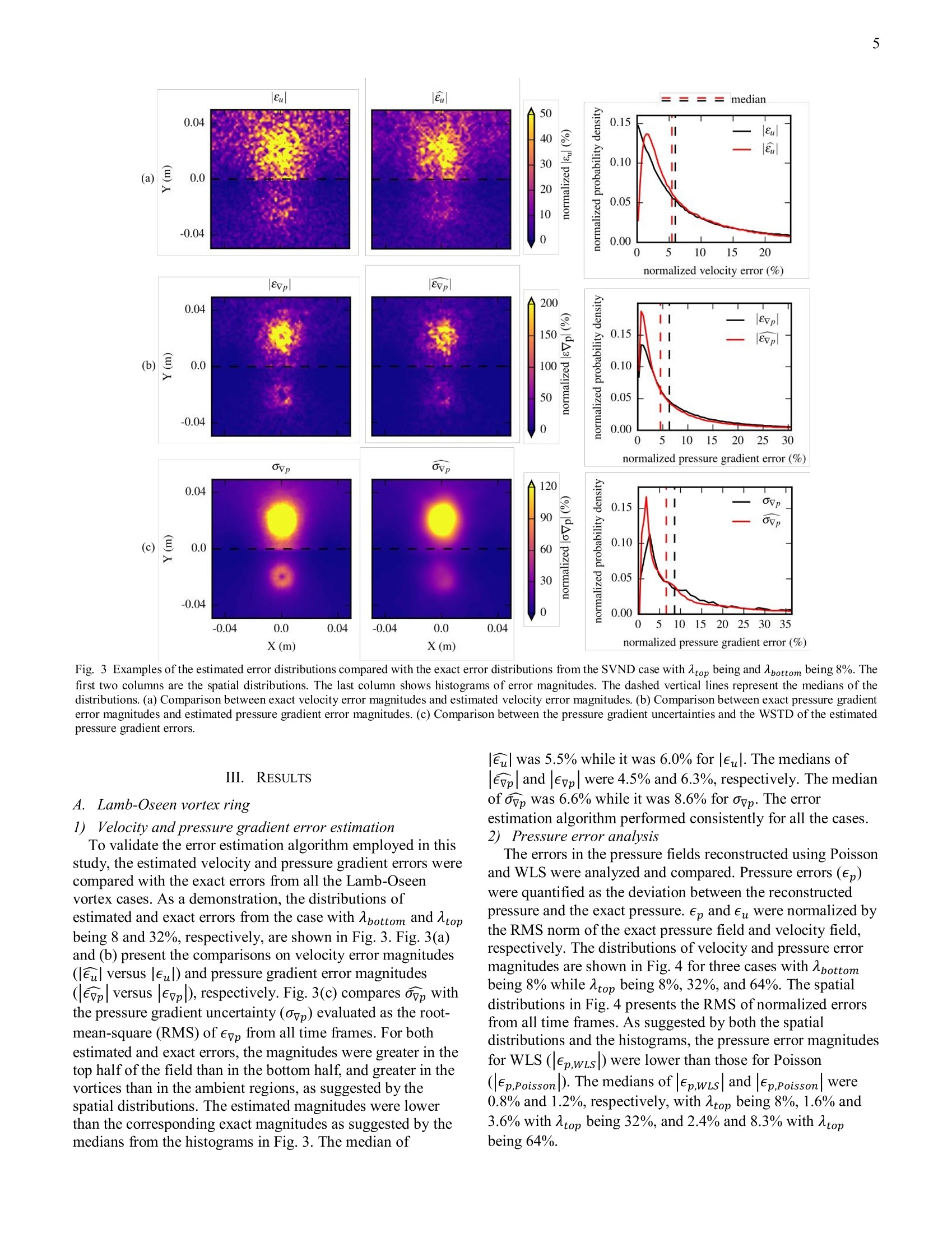
方案详情
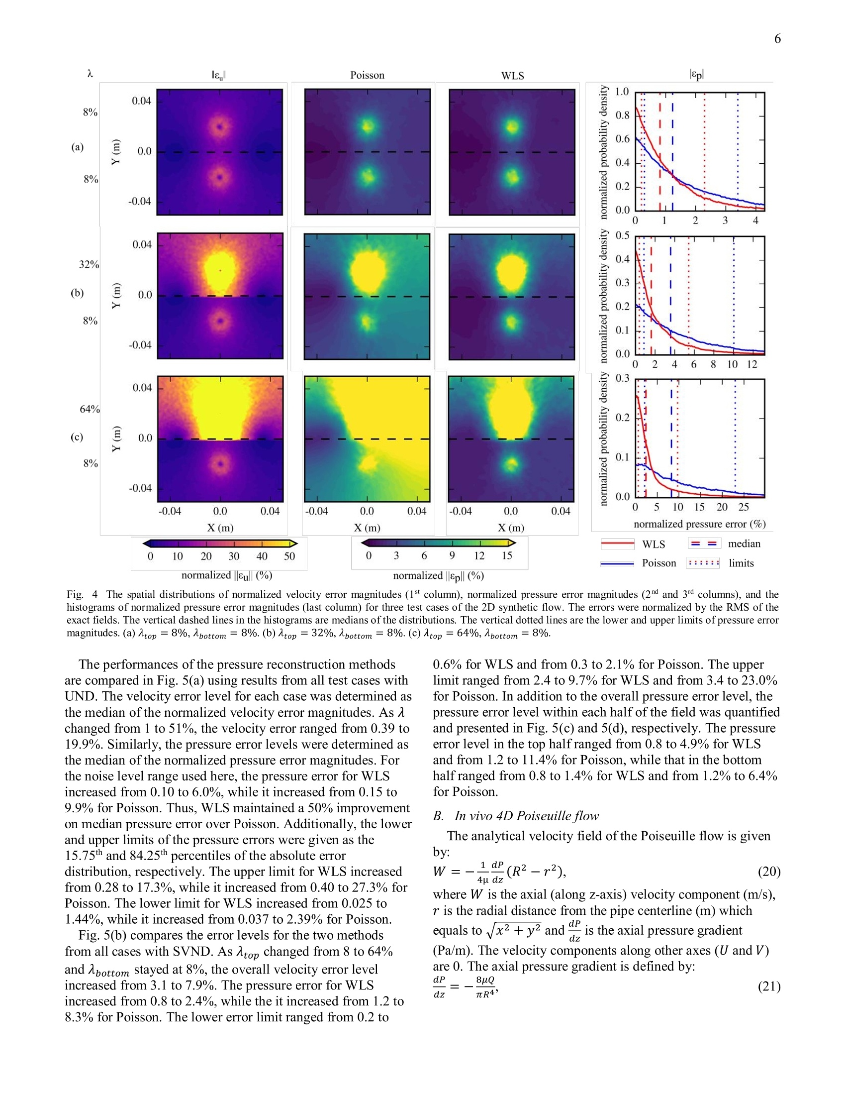
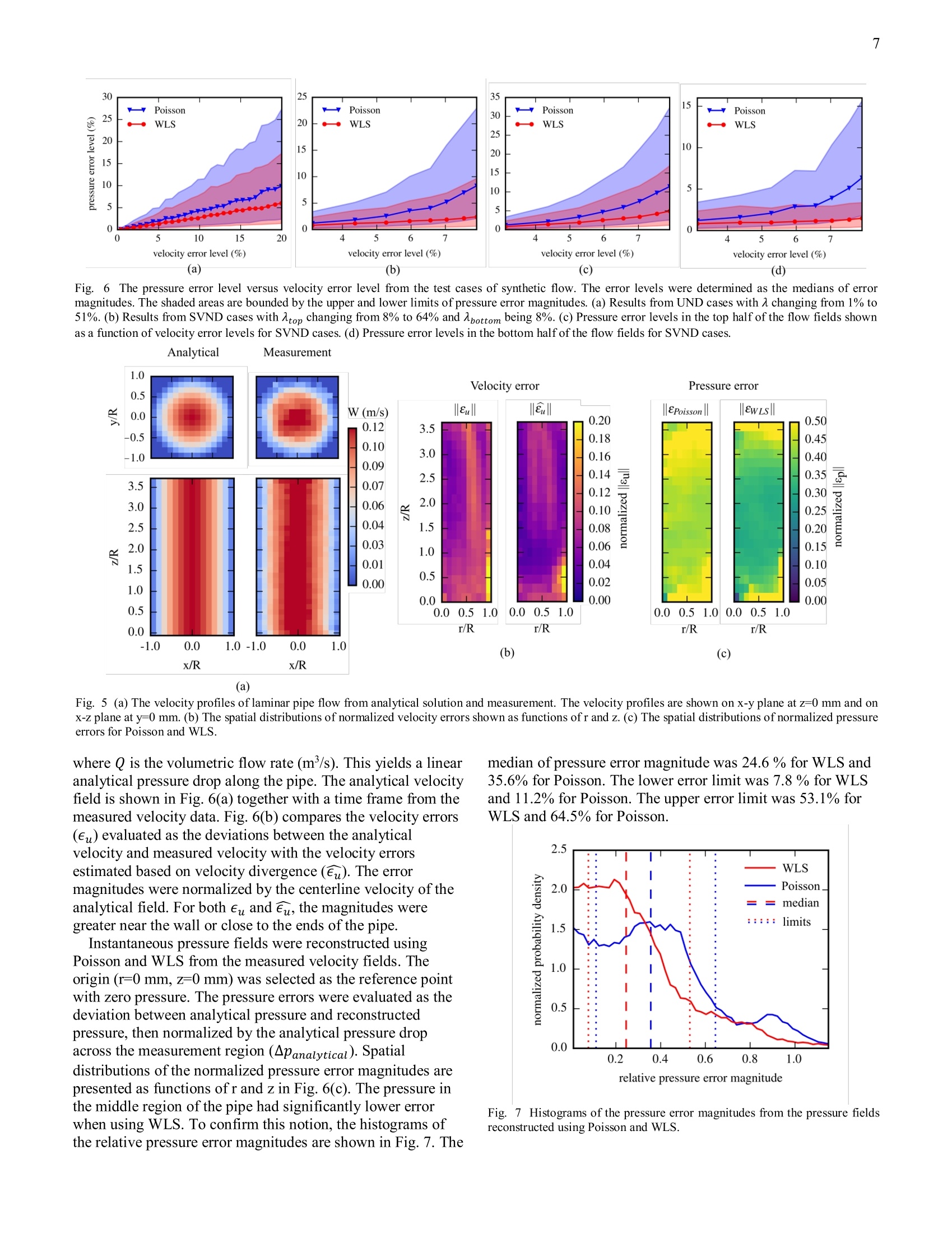
文
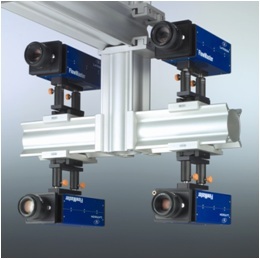
采用LaVision新近推出的DaVis10.0图像数据采集和处理分析软件平台,对脑动脉瘤模型内血液流动的磁共振成像数据进行抖盒子处理(STB),获得了模型中流体的四维流场信息,并利用这一结果,进行了压力求解。
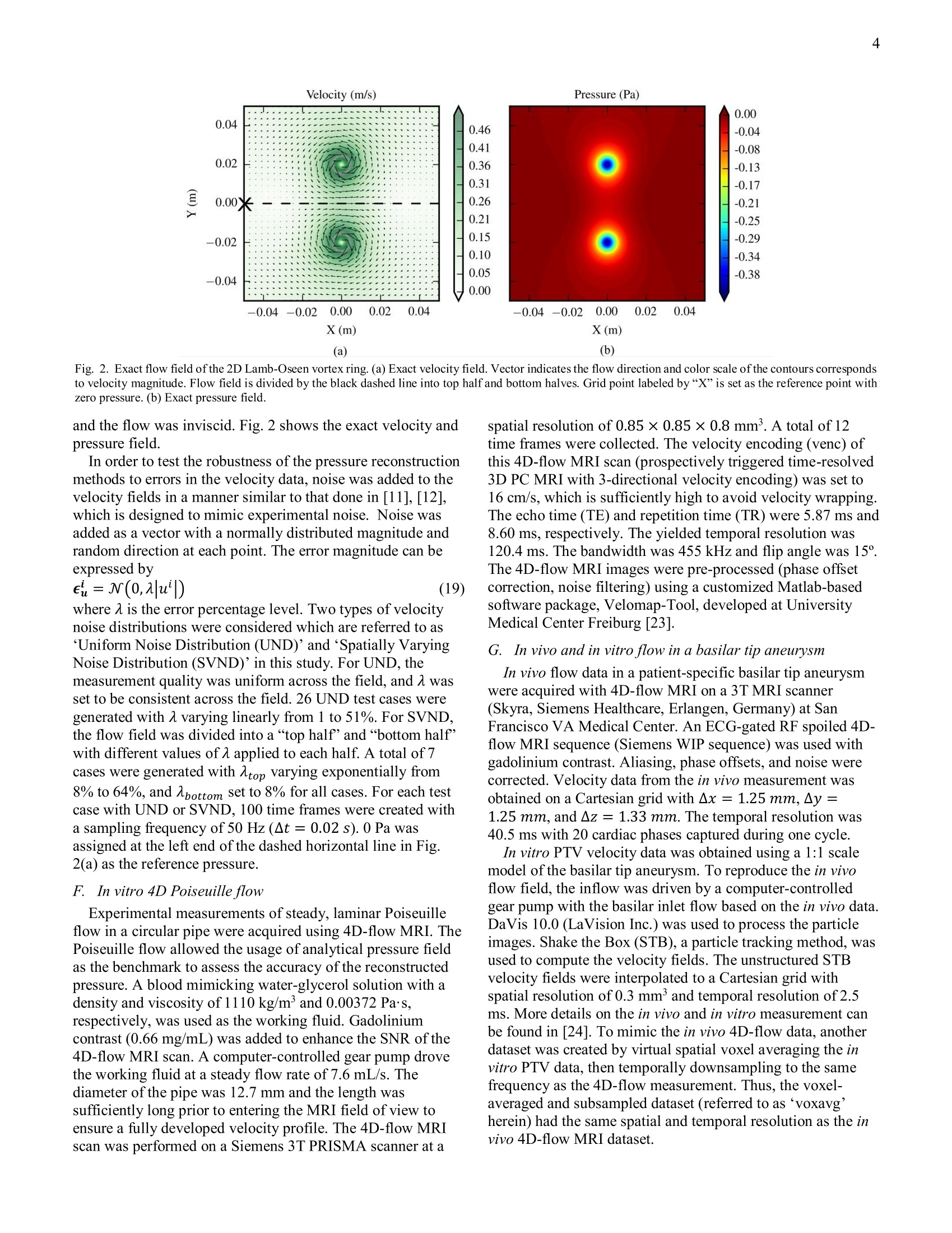
方案详情

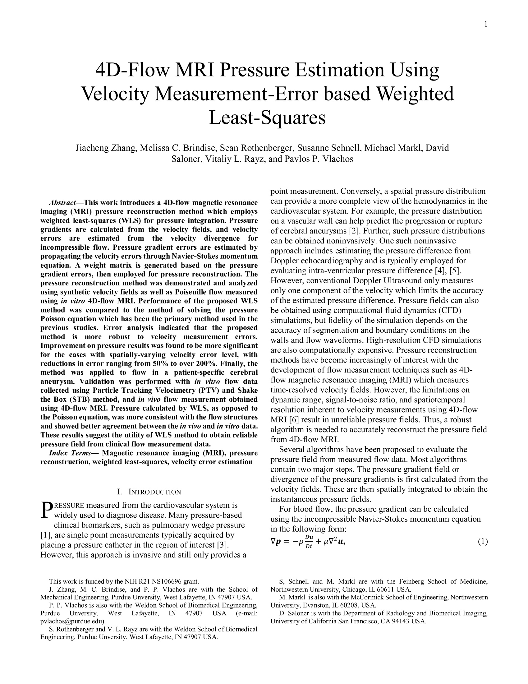
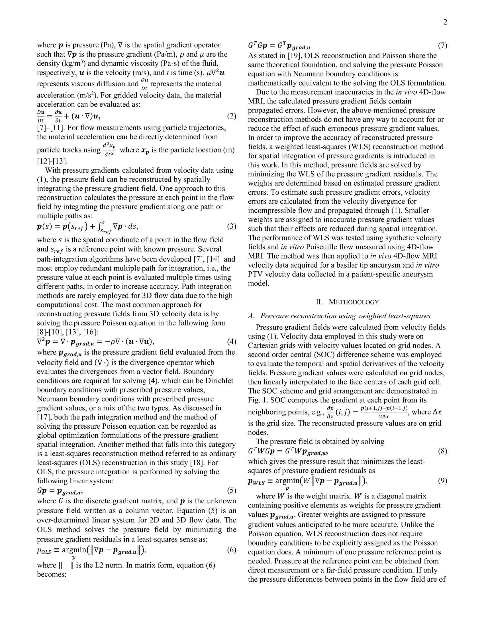
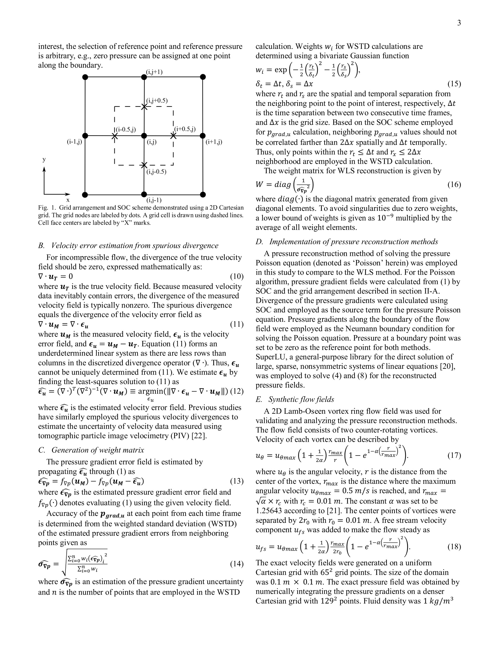
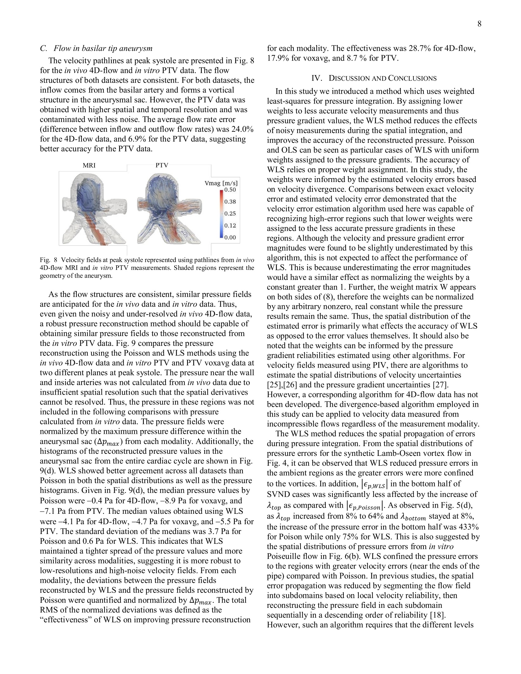
5 10 This work has been submitted to the IEEE for possible publication. Copyright may be transferredwithout notice, after which this version may no longer be accessible. 4D-Flow MRI Pressure Estimation UsingVelocity Measurement-Error based WeightedLeast-Squares Jiacheng Zhang, Melissa C. Brindise, Sean Rothenberger, Susanne Schnell, Michael Markl, DavidSaloner, Vitaliy L. Rayz, and Pavlos P. Vlachos Abstract—This work introduces a 4D-flow magnetic resonanceimaging (MRI) pressure reconstruction method which employsweighted least-squares (WLS) for pressure integration. Pressuregradients are calculated from the velocity fields, and velocityerrors areestimated fromthe velocity(divergence forincompressible flow. Pressure gradient errors are estimated bypropagating the velocity errors through Navier-Stokes momentumequation. A weight matrix is generated based on the pressuregradient errors, then employed for pressure reconstruction. Thepressure reconstruction method was demonstrated and analyzedusing synthetic velocity fields as well as Poiseuille flow measuredusing in vitro 4D-flow MRI. Performance of the proposed WLSmethod was compared to the method of solving the pressurePoisson equation which has been the primary method used in theprevious studies. Error analysis indicated that the proposedmethod is more robust to velocity measurement errors.Improvement on pressure results was found to be more significantfor the cases with spatially-varying velocity error level, withreductions in error ranging from 50% to over 200%. Finally, themethodwas applied to flow in aa patient-specific cerebralaneurysm. Validation was performed with in vitro flow datacollected using Particle Tracking Velocimetry (PTV) and Shakethe Box (STB) method, and in vivo flow measurement obtainedusing 4D-flow MRI.Pressure calculated by WLS, as opposed tothe Poisson equation, was more consistent with the flow structuresand showed better agreement between the in vivo and in vitro data.These results suggest the utility of WLS method to obtain reliablepressure field from clinical flow measurement data. Index Terms— Magnetic resonance imaging (MRI), pressurereconstruction, weighted least-squares, velocity error estimation 1.IINTRODUCTION RESSURE measured from the cardiovascular system isP.widely used to diagnose disease. Many pressure-basedclinical biomarkers, such as pulmonary wedge pressure [1], are single point measurements typically acquired by placing a pressure catheter in the region of interest [3]. However, this approach is invasive and still only provides a This work is funded by the NIH R21 NS106696 grant. ( J. Zhang, M . C. Brindise, and P . P . V l achos ar e wi t h th e Sc h ool ofMechanical E n gineering, Purdue Unversity, West Lafa y ette, IN 47907 USA . ) ( P . P. Vlachos is also with the Weldon School o f B iomedical Engineering,Purdue Unversity, West Lafayette, IN 47907 USA (e-mail: pvlachos@purdue.edu). ) ( S. Rothenberger and V. L. Rayz are with the Weldon School of Biomedical Engineering, Purdue Unversity, West L a fayette, IN 4 7 907 USA. ) point measurement. Conversely, a spatial pressure distributioncan provide a more complete view of the hemodynamics in thecardiovascular system. For example, the pressure distributionon a vascular wall can help predict the progression or ruptureof cerebral aneurysms [2]. Further, such pressure distributionscan be obtained noninvasively. One such noninvasiveapproach includes estimating the pressure difference fromDoppler echocardiography and is typically employed forevaluating intra-ventricular pressure difference [4], [5].However, conventional Doppler Ultrasound only measuresonly one component of the velocity which limits the accuracyof the estimated pressure difference. Pressure fields can alsobe obtained using computational fluid dynamics (CFD)simulations, but fidelity of the simulation depends on theaccuracy of segmentation and boundary conditions on thewalls and flow waveforms. High-resolution CFD simulationsare also computationally expensive. Pressure reconstructionmethods have become increasingly of interest with thedevelopment of flow measurement techniques such as 4D-flow magnetic resonance imaging (MRI) which measurestime-resolved velocity fields. However, the limitations ondynamic range, signal-to-noise ratio, and spatiotemporalresolution inherent to velocity measurements using 4D-flowMRI [6] result in unreliable pressure fields. Thus, a robustalgorithm is needed to accurately reconstruct the pressure fieldfrom 4D-flow MRI. Several algorithms have been proposed to evaluate thepressure field from measured flow data. Most algorithmscontain two major steps. The pressure gradient field ordivergence of the pressure gradients is first calculated from thevelocity fields. These are then spatially integrated to obtain theinstantaneous pressure fields. For blood flow, the pressure gradient can be calculatedusing the incompressible Navier-Stokes momentum equationin the following form: V p = - p u + u V 2 u , (1) ( S, Schnell and M . Markl a r e w i th t h e F e inberg School of Me d icine, Northwestern University, Chicago, IL 60611 USA. ) M. Markl is also with the McCormick School ofEngineering, NorthwesternUniversity, Evanston, IL 60208, USA. D. Saloner is with the Department of Radiology and Biomedical Imaging,University of California San Francisco, CA 94143 USA. where p is pressure (Pa), V is the spatial gradient operatorsuch that Vp is the pressure gradient (Pa/m), p and u are thedensity (kg/m’) and dynamic viscosity (Pas) of the fluid,respectively, u is the velocity (m/s), and t is time (s). uVurepresents viscous diffusion andDud-represents the materialacceleration (m/s). For gridded velocity data, the materialacceleration can be evaluated as: [7]-[11]. For flow measurements using particle trajectories,the material acceleration can be directly determined fromparticle tracks using “ where x,, is the particle location (m)[12]-[13]. With pressure gradients calculated from velocity data using(1), the pressure field can be reconstructed by spatiallyintegrating the pressure gradient field. One approach to thisreconstruction calculates the pressure at each point in the flowfield by integrating the pressure gradient along one path ormultiple paths as: where s is the spatial coordinate of a point in the flow field and Sref is a reference point with known pressure. Severalpath-integration algorithms have been developed [7],[14] andmost employ redundant multiple path for integration, i.e., thepressure value at each point is evaluated multiple times usingdifferent paths, in order to increase accuracy. Path integrationmethods are rarely employed for 3D flow data due to the highcomputational cost. The most common approach forreconstructing pressure fields from 3D velocity data is by solving the pressure Poisson equation in the following form[8]-[10],[13],[16]: where pgradu is the pressure gradient field evaluated from thevelocity field and (V·) is the divergence operator whichevaluates the divergences from a vector field. Boundaryconditions are required for solving (4),which can be Dirichletboundary conditions with prescribed pressure values,Neumann boundary conditions with prescribed pressuregradient values, or a mix of the two types. As discussed in[17], both the path integration method and the method ofsolving the pressure Poisson equation can be regarded asglobal optimization formulations of the pressure-gradientspatial integration. Another method that falls into this categoryis a least-squares reconstruction method referred to as ordinaryleast-squares (OLS) reconstruction in this study [18]. ForOLS, the pressure integration is performed by solving thefollowing linear system: where G is the discrete gradient matrix, and p is the unknownpressure field written as a column vector. Equation (5) is anover-determined linear system for 2D and 3D flow data. TheOLS method solves the pressure field by minimizing thepressure gradient residuals in a least-squares sense as: whereis the L2 norm. In matrix form, equation (6)becomes: As stated in [19], OLS reconstruction and Poisson share the same theoretical foundation, and solving the pressure Poisson equation with Neumann boundary conditions is mathematically equivalent to the solving the OLS formulation.Due to the measurement inaccuracies in the in vivo 4D-flowMRI, the calculated pressure gradient fields containpropagated errors. However, the above-mentioned pressurereconstruction methods do not have any way to account for orreduce the effect of such erroneous pressure gradient values.In order to improve the accuracy of reconstructed pressurefields, a weighted least-squares (WLS) reconstruction methodfor spatial integration of pressure gradients is introduced inthis work. In this method, pressure fields are solved byminimizing the WLS of the pressure gradient residuals. Theweights are determined based on estimated pressure gradienterrors. To estimate such pressure gradient errors, velocityerrors are calculated from the velocity divergence forincompressible flow and propagated through (1). Smallerweights are assigned to inaccurate pressure gradient valuessuch that their effects are reduced during spatial integration.The performance of WLS was tested using synthetic velocityfields and in vitro Poiseuille flow measured using 4D-flowMRI. The method was then applied to in vivo 4D-flow MRIvelocity data acquired for a basilar tip aneurysm and in vitroPTV velocity data collected in a patient-specific aneurysmmodel. II. METHODOLOGY A.Pressure reconstruction using weighted least-squares Pressure gradient fields were calculated from velocity fieldsusing (1). Velocity data employed in this study were onCartesian grids with velocity values located on grid nodes. Asecond order central (SOC) difference scheme was employedto evaluate the temporal and spatial derivatives of the velocityfields. Pressure gradient values were calculated on grid nodes,then linearly interpolated to the face centers ofeach grid cell.The SOC scheme and grid arrangement are demonstrated inFig. 1. SOC computes the gradient at each point from itsneighboring points, e.g.,(i(,ij,j)=e(i+1))-p(i-12, where A2Axis the grid size. The reconstructed pressure values are on gridnodes. The pressure field is obtained by solving GWGp=G’Wpgrad,u (8)which gives the pressure result that minimizes the least-squares of pressure gradient residuals as p where W is the weight matrix. W is a diagonal matrixcontaining positive elements as weights for pressure gradientvalues p grad,u. Greater weights are assigned to pressuregradient values anticipated to be more accurate. Unlike thePoisson equation, WLS reconstruction does not requireboundary conditions to be explicitly assigned as the Poissonequation does. A minimum of one pressure reference point isneeded. Pressure at the reference point can be obtained fromdirect measurement or a far-field pressure condition. Ifonlythe pressure differences between points in the flow field are of interest, the selection of reference point and reference pressureis arbitrary, e.g., zero pressure can be assigned at one pointalong the boundary. V Fig. 1. Grid arrangement and SOC scheme demonstrated using a 2D Cartesiangrid. The grid nodes are labeled by dots. A grid cell is drawn using dashed lines.Cell face centers are labeled by“X" marks. B. Velocity error estimation from spurious divergence For incompressible flow, the divergence of the true velocityfield should be zero, expressed mathematically as:(10) V·ur=0 where ur is the true velocity field. Because measured velocitydata inevitably contain errors, the divergence of the measuredvelocity field is typically nonzero. The spurious divergenceequals the divergence of the velocity error field as V·uM=V.E (11) where um is the measured velocity field, Eu is the velocity error field, and eu=uM -up. Equation (11) forms anunderdetermined linear system as there are less rows thancolumns in the discretized divergence operator (V). Thus, eucannot be uniquely determined from (11). We estimate Eu byfinding the least-squares solution to (11) as eu=(V.)"(V2)-1(V·uM)= argmin(|V·Eu-·uMll) (12)Eu wheree is the estimated velocity error field. Previous studieshave similarly employed the spurious velocity divergences toestimate the uncertainty of velocity data measured usingtomographic particle image velocimetry (PIV) [22]. C. Generation of weight matrixThe pressure gradient error field is estimated bypropagating through (1) asEvp=fvp(uM)-fvp(uM-e) (13) where Evp is the estimated pressure gradient error field andfvp () denotes evaluating (1) using the given velocity field. Accuracy of the Pgrad,u at each point from each time frameis determined from the weighted standard deviation (WSTD)of the estimated pressure gradient errors from neighboringpoints given as where dvp is an estimation of the pressure gradient uncertaintyand n is the number of points that are employed in the WSTD calculation. Weights w; for WSTD calculations aredetermined using a bivariate Gaussian function where rrand r, are the spatial and temporal separation fromthe neighboring point to the point of interest, respectively, Atis the time separation between two consecutive time frames,and Ax is the grid size. Based on the SOC scheme employedfor pgrad,u calculation, neighboring Pgrad,u values should notbe correlated farther than 2Ax spatially and At temporally.Thus, only points within the rt ≤ At andre ≤ 2Ax neighborhood are employed in the WSTD calculation. The weight matrix for WLS reconstruction is given by where diag() is the diagonal matrix generated from givendiagonal elements. To avoid singularities due to zero weights,a lower bound of weights is given as 10-°multiplied by theaverage of all weight elements. D. Implementation ofpressure reconstruction methods A pressure reconstruction method of solving the pressurePoisson equation (denoted as Poisson’herein) was employedin this study to compare to the WLS method. For the Poissonalgorithm, pressure gradient fields were calculated from (1) bySOC and the grid arrangement described in section II-A.Divergence of the pressure gradients were calculated usingSOC and employed as the source term for the pressure Poissonequation. Pressure gradients along the boundary of the flowfield were employed as the Neumann boundary condition forsolving the Poisson equation. Pressure at a boundary point wasset to be zero as the reference point for both methods.SuperLU, a general-purpose library for the direct solution oflarge, sparse, nonsymmetric systems of linear equations [20],was employed to solve (4) and (8) for the reconstructedpressure fields. E..Synthetic flow fields A 2D Lamb-Oseen vortex ring flow field was used forvalidating and analyzing the pressure reconstruction methods.The flow field consists of two counter-rotating vortices.Velocity of each vortex can be described by (a) (b) Fig. 2. Exact flow field of the 2D Lamb-Oseen vortex ring. (a) Exact velocity field. Vector indicates the flow direction and color scale of the contours correspondsto velocity magnitude. Flow field is divided by the black dashed line into top half and bottom halves.Grid point labeled by “X”is set as the reference point withzero pressure. (b) Exact pressure field. and the flow was inviscid. Fig. 2 shows the exact velocity andpressure field. In order to test the robustness of the pressure reconstructionmethods to errors in the velocity data, noise was added to thevelocity fields in a manner similar to that done in [11],[12],which is designed to mimic experimental noise. Noise wasadded as a vector with a normally distributed magnitude andrandom direction at each point. The error magnitude can beexpressed by where a is the error percentage level. Two types of velocitynoise distributions were considered which are referred to as‘Uniform Noise Distribution (UND)'and‘Spatially VaryingNoise Distribution (SVND)’in this study. For UND, themeasurement quality was uniform across the field, and A wasset to be consistent across the field. 26 UND test cases weregenerated with A varying linearly from 1 to 51%. For SVND,the flow field was divided into a“top half’and “bottom half'with different values of applied to each half. A total of 7cases were generated with Atop varying exponentially from8% to 64%, and Abottom set to 8% for all cases. For each testcase with UND or SVND, 100 time frames were created witha sampling frequency of 50 Hz (At= 0.02 s). 0 Pa wasassigned at the left end of the dashed horizontal line in Fig.2(a) as the reference pressure. F. I1n vitro 4D Poiseuille flow Experimental measurements of steady, laminar Poiseuilleflow in a circular pipe were acquired using 4D-flow MRI. ThePoiseuille flow allowed the usage of analytical pressure fieldas the benchmark to assess the accuracy of the reconstructedpressure. A blood mimicking water-glycerol solution with adensity and viscosity of 1110 kg/m’and 0.00372 Pas,respectively, was used as the working fluid. Gadoliniumcontrast (0.66 mg/mL) was added to enhance the SNR of the4D-flow MRI scan. A computer-controlled gear pump drovethe working fluid at a steady flow rate of 7.6 mL/s. Thediameter of the pipe was 12.7 mm and the length wassufficiently long prior to entering the MRI field of view toensure a fully developed velocity profile. The 4D-flow MRIscan was performed on a Siemens 3T PRISMA scanner at a spatial resolution of 0.85 ×0.85×0.8 mm. A total of 12time frames were collected. The velocity encoding (venc) ofthis 4D-flow MRI scan (prospectively triggered time-resolved3D PC MRI with 3-directional velocity encoding) was set to16 cm/s, which is sufficiently high to avoid velocity wrapping.The echo time (TE) and repetition time (TR) were 5.87 ms and8.60 ms, respectively.The yielded temporal resolution was120.4 ms. The bandwidth was 455 kHz and flip angle was 15°.The 4D-flow MRI images were pre-processed (phase offsetcorrection, noise filtering) using a customized Matlab-basedsoftware package, Velomap-Tool, developed at UniversityMedical Center Freiburg [23]. G. In vivo and in vitro flow in a basilar tip aneurysm In vivo flow data in a patient-specific basilar tip aneurysmwere acquired with 4D-flow MRI on a 3T MRI scanner(Skyra, Siemens Healthcare, Erlangen, Germany) at SanFrancisco VA Medical Center. An ECG-gated RF spoiled 4D-flow MRI sequence (Siemens WIP sequence) was used withgadolinium contrast. Aliasing, phase offsets, and noise werecorrected. Velocity data from the in vivo measurement wasobtained on a Cartesian grid with Ax=1.25 mm, Ay=1.25 mm, and Az= 1.33 mm. The temporal resolution was40.5 ms with 20 cardiac phases captured during one cycle. In vitro PTV velocity data was obtained using a 1:1 scalemodel of the basilar tip aneurysm. To reproduce the in vivoflow field, the inflow was driven by a computer-controlledgear pump with the basilar inlet flow based on the in vivo data.DaVis 10.0 (LaVision Inc.) was used to process the particleimages. Shake the Box (STB), a particle tracking method, wasused to compute the velocity fields. The unstructured STBvelocity fields were interpolated to a Cartesian grid withspatial resolution of 0.3 mm’and temporal resolution of 2.5ms. More details on the in vivo and in vitro measurement canbe found in [24]. To mimic the in vivo 4D-flow data, anotherdataset was created by virtual spatial voxel averaging the invitro PTV data, then temporally downsampling to the samefrequency as the 4D-flow measurement. Thus, the voxel-averaged and subsampled dataset (referred to as ‘voxavg’herein) had the same spatial and temporal resolution as the invivo 4D-flow MRI dataset. Fig. 3 Examples of the estimated error distributions compared with the exact error distributions from the SVND case with Atop being and Abottom being 8%. Thefirst two columns are the spatial distributions. The last column shows histograms of error magnitudes. The dashed vertical lines represent the medians of thedistributions. (a) Comparison between exact velocity error magnitudes and estimated velocity error magnitudes.(b) Comparison between exact pressure gradienterror magnitudes and estimated pressure gradient error magnitudes. (c) Comparison between the pressure gradient uncertainties and the WSTD of the estimatedpressure gradient errors. III.RESULTS 4. Lamb-Oseen vortex ring 1))Velocity and pressure gradient error estimation To validate the error estimation algorithm employed in thisstudy, the estimated velocity and pressure gradient errors werecompared with the exact errors from all the Lamb-Oseenvortex cases. As a demonstration, the distributions ofestimated and exact errors from the case with Abottom and Atopbeing 8 and 32%, respectively, are shown in Fig. 3. Fig. 3(a)and (b) present the comparisons on velocity error magnitudes(leul versus eul) and pressure gradient error magnitudes(|evp| versus |evp|), respectively. Fig. 3(c) compares ovp withthe pressure gradient uncertainty (vp) evaluated as the root-mean-square (RMS) of Ev from all time frames. For bothestimated and exact errors, the magnitudes were greater in thetop half of the field than in the bottom half, and greater in thevortices than in the ambient regions, as suggested by thespatial distributions. The estimated magnitudes were lowerthan the corresponding exact magnitudes as suggested by themedians from the histograms in Fig. 3. The median of |e| was 5.5% while it was 6.0% for |eul. The medians ofevp and Evp were 4.5% and 6.3%, respectively. The medianof ov, was 6.6% while it was 8.6% for ovp. The errorestimation algorithm performed consistently for all the cases. 2)Pressure error analysis The errors in the pressure fields reconstructed using Poissonand WLS were analyzed and compared. Pressure errors (E,)were quantified as the deviation between the reconstructedpressure and the exact pressure. e, and eu were normalized bythe RMS norm of the exact pressure field and velocity field,respectively. The distributions of velocity and pressure errormagnitudes are shown in Fig. 4 for three cases with Abottombeing 8% while Atop being 8%, 32%, and 64%. The spatialdistributions in Fig. 4 presents the RMS of normalized errorsfrom all time frames. As suggested by both the spatialdistributions and the histograms, the pressure error magnitudesfor WLS (|ep,wLs|) were lower than those for Poisson(Ep,Poisson ). The medians of Ep,wis and Ep,Poisson were0.8% and 1.2%, respectively, with Atop being 8%, 1.6% and3.6% with Atop being 32%, and 2.4% and 8.3% with Atopbeing 64%. Fig..44The spatial distributions of normalized velocity error magnitudes (1*t column), normalized pressure error magnitudes (2"d and 3rd columns), and thehistograms of normalized pressure error magnitudes (last column) for three test cases of the 2D synthetic flow. The errors were normalized by the RMS of theexact fields. The vertical dashed lines in the histograms are medians of the distributions. The vertical dotted lines are the lower and upper limits of pressure errormagnitudes. (a) Atop =8%, Abottom=8%. (b) Atop=32%,Abottom=8%. (c) Atop =64%,Abottom =8%. The performances of the pressure reconstruction methods are compared in Fig. 5(a) using results from all test cases withUND. The velocity error level for each case was determined asthe median ofthe normalized velocity error magnitudes. As Achanged from 1 to 51%, the velocity error ranged from 0.39 to19.9%. Similarly, the pressure error levels were determined asthe median of the normalized pressure error magnitudes. Forthe noise level range used here, the pressure error for WLSincreased from 0.10 to 6.0%, while it increased from 0.15 to9.9% for Poisson. Thus, WLS maintained a 50% improvementon median pressure error over Poisson. Additionally, the lowerand upper limits of the pressure errors were given as the15.75th and 84.25h percentiles ofthe absolute errordistribution, respectively. The upper limit for WLS increasedfrom 0.28 to 17.3%, while it increased from 0.40 to 27.3% forPoisson. The lower limit for WLS increased from 0.025 to1.44%, while it increased from 0.037 to2.39% for Poisson.Fig. 5(b) compares the error levels for the two methodsfrom all cases with SVND. As Atop changed from 8 to 64%and Abottom stayed at 8%, the overall velocity error levelincreased from 3.1 to 7.9%. The pressure error for WLSincreased from 0.8 to 2.4%, while the it increased from 1.2 to8.3% for Poisson. The lower error limit ranged from 0.2 to 0.6% for WLS and from 0.3 to 2.1% for Poisson. The upperlimit ranged from 2.4 to 9.7% for WLS and from 3.4 to 23.0%for Poisson.In addition to the overall pressure error level, thepressure error level within each half of the field was quantifiedand presented in Fig. 5(c) and 5(d), respectively. The pressureerror level in the top half ranged from 0.8 to 4.9% for WLSand from 1.2 to 11.4% for Poisson, while that in the bottomhalf ranged from 0.8 to 1.4% for WLS and from 1.2% to 6.4%for Poisson. B.In vivo 4D Poiseuille flow The analytical velocity field of the Poiseuille flow is givenby: where W is the axial (along z-axis) velocity component (m/s),r is the radial distance from the pipe centerline (m) whichdPequals tox2+y2 and is the axial pressure gradient (Pa/m). The velocity components along other axes (U and V)are 0. The axial pressure gradient is defined by: Fig. 6 The pressure error level versus velocity error level from the test cases of synthetic flow. The error levels were determined as the medians of errormagnitudes. The shaded areas are bounded by the upper and lower limits of pressure error magnitudes. (a) Results from UND cases with 1 changing from 1% to51%. (b) Results from SVND cases with Atop changing from 8% to 64% and Abottom being 8%. (c) Pressure error levels in the top half of the flow fields shownas a function of velocity error levels for SVND cases. (d) Pressure error levels in the bottom half of the flow fields for SVND cases. Analytical Measurement (a) Fig. 5 (a) The velocity profiles of laminar pipe flow from analytical solution and measurement. The velocity profiles are shown on x-y plane at z=0 mm and onx-z plane at y=0 mm. (b) The spatial distributions of normalized velocity errors shown as functions of r and z. (c) The spatial distributions of normalized pressureerrors for Poisson and WLS. where Q is the volumetric flow rate (m’/s). This yields a linearanalytical pressure drop along the pipe. The analytical velocityfield is shown in Fig.6(a) together with a time frame from themeasured velocity data. Fig. 6(b) compares the velocity errors(Eu) evaluated as the deviations between the analyticalvelocity and measured velocity with the velocity errorsestimated based on velocity divergence (E). The errormagnitudes were normalized by the centerline velocity of theanalytical field. For both eu and eu, the magnitudes weregreater near the wall or close to the ends of the pipe. Instantaneous pressure fields were reconstructed usingPoisson and WLS from the measured velocity fields. Theorigin (r=0 mm, z=0 mm) was selected as the reference pointwith zero pressure. The pressure errors were evaluated as thedeviation between analytical pressure and reconstructedpressure, then normalized by the analytical pressure dropacross the measurement region (Apanalytical). Spatialdistributions of the normalized pressure error magnitudes arepresented as functions ofr and z in Fig.6(c). The pressure inthe middle region of the pipe had significantly lower errorwhen using WLS. To confirm this notion, the histograms ofthe relative pressure error magnitudes are shown in Fig. 7. The median of pressure error magnitude was 24.6 % for WLS and35.6% for Poisson. The lower error limit was 7.8 % for WLSand 11.2% for Poisson. The upper error limit was 53.1% forWLS and 64.5%for Poisson. Fig.7 Histograms of the pressure error magnitudes from the pressure fieldsreconstructed using Poisson and WLS. The velocity pathlines at peak systole are presented in Fig. 8for the in vivo 4D-flow and in vitro PTV data. The flowstructures of both datasets are consistent. For both datasets, theinflow comes from the basilar artery and forms a vorticalstructure in the aneurysmal sac. However, the PTV data wasobtained with higher spatial and temporal resolution and wascontaminated with less noise. The average flow rate error(difference between inflow and outflow flow rates) was 24.0%for the 4D-flow data, and 6.9% for the PTV data, suggestingbetter accuracy for the PTV data. Fig. 8 Velocity fields at peak systole represented using pathlines from in vivo4D-flow MRI and in vitro PTV measurements. Shaded regions represent thegeometry of the aneurysm. As the flow structures are consistent, similar pressure fieldsare anticipated for the in vivo data and in vitro data. Thus,even given the noisy and under-resolved in vivo 4D-flow data,a robust pressure reconstruction method should be capable ofobtaining similar pressure fields to those reconstructed fromthe in vitro PTV data. Fig. 9 compares the pressurereconstruction using the Poisson and WLS methods using thein vivo 4D-flow data and in vitro PTV and PTV voxavg data attwo different planes at peak systole. The pressure near the walland inside arteries was not calculated from in vivo data due toinsufficient spatial resolution such that the spatial derivativescannot be resolved. Thus, the pressure in these regions was notincluded in the following comparisons with pressurecalculated from in vitro data. The pressure fields werenormalized by the maximum pressure difference within theaneurysmal sac (Apmax) from each modality. Additionally, thehistograms of the reconstructed pressure values in theaneurysmal sac from the entire cardiac cycle are shown in Fig.9(d). WLS showed better agreement across all datasets thanPoisson in both the spatial distributions as well as the pressurehistograms. Given in Fig. 9(d), the median pressure values byPoisson were -0.4 Pa for 4D-flow, -8.9 Pa for voxavg, and-7.1 Pa from PTV. The median values obtained using WLSwere -4.1 Pa for 4D-flow,-4.7 Pa for voxavg, and -5.5 Pa forPTV. The standard deviation of the medians was 3.7 Pa forPoisson and 0.6 Pa for WLS. This indicates that WLSmaintained a tighter spread of the pressure values and moresimilarity across modalities, suggesting it is more robust tolow-resolutions and high-noise velocity fields. From eachmodality, the deviations between the pressure fieldsreconstructed by WLS and the pressure fields reconstructed byPoisson were quantified and normalized by Apmax. The totalRMS of the normalized deviations was defined as the“effectiveness”of WLS on improving pressure reconstruction for each modality. The effectiveness was 28.7% for 4D-flow,17.9% for voxavg, and 8.7% for PTV. IV. DISCUSSION AND CONCLUSIONS In this study we introduced a method which uses weighted least-squares for pressure integration. By assigning lowerweights to less accurate velocity measurements and thuspressure gradient values, the WLS method reduces the effectsof noisy measurements during the spatial integration, andimproves the accuracy of the reconstructed pressure.Poissonand OLS can be seen as particular cases of WLS with uniformweights assigned to the pressure gradients. The accuracy ofWLS relies on proper weight assignment. In this study, theweights were informed by the estimated velocity errors basedon velocity divergence. Comparisons between exact velocityerror and estimated velocity error demonstrated that thevelocity error estimation algorithm used here was capable ofrecognizing high-error regions such that lower weights wereassigned to the less accurate pressure gradients in theseregions. Although the velocity and pressure gradient errormagnitudes were found to be slightly underestimated by thisalgorithm, this is not expected to affect the performance ofWLS. This is because underestimating the error magnitudeswould have a similar effect as normalizing the weights by aconstant greater than 1. Further, the weight matrix W appearson both sides of (8), therefore the weights can be normalizedby any arbitrary nonzero, real constant while the pressureresults remain the same. Thus, the spatial distribution of theestimated error is primarily what effects the accuracy of WLSas opposed to the error values themselves. It should also benoted that the weights can be informed by the pressuregradient reliabilities estimated using other algorithms. Forvelocity fields measured using PIV, there are algorithms toestimate the spatial distributions of velocity uncertainties[25],[26] and the pressure gradient uncertainties [27].However, a corresponding algorithm for 4D-flow data has notbeen developed. The divergence-based algorithm employed inthis study can be applied to velocity data measured fromincompressible flows regardless of the measurement modality. The WLS method reduces the spatial propagation of errors during pressure integration. From the spatial distributions of pressure errors for the synthetic Lamb-Oseen vortex flow in Fig. 4, it can be observed that WLS reduced pressure errors in the ambient regions as the greater errors were more confined to the vortices. In addition, Ep,WLs in the bottom half of SVND cases was significantly less affected by the increase of Atop as compared with Ep,Poisson. As observed in Fig. 5(d), as ltop increased from 8% to 64% and Abottom stayed at 8%, the increase of the pressure error in the bottom half was 433% for Poison while only 75% for WLS. This is also suggested by the spatial distributions of pressure errors from in vitro Poiseuille flow in Fig. 6(b). WLS confined the pressure errors to the regions with greater velocity errors (near the ends of the pipe) compared with Poisson. In previous studies, the spatial error propagation was reduced by segmenting the flow field into subdomains based on local velocity reliability, then reconstructing the pressure field in each subdomain sequentially in a descending order of reliability [18]. However, such an algorithm requires that the different levels Fig. 9. Spatial and probability density distributions of pressure fields reconstructed using Poisson and WLS from each dataset. The spatial distributions arepresented by the normalized pressure values on a x-y plane and a y-z plane cutting through the aneurysm sac at peak systole. Shaded regions correspond to thegeometry of the aneurysm. (a) Spatial distributions for in vivo 4D-flow MRI data. (b) Spatial distributions for voxel-averaged (voxavg) PTV data. (c) Spatialdistributions for in vitro PTV data.(d) Probability density distributions ofthe reconstructed pressure values within the aneurysmal sac. of measurement reliability are spatially separable in the flowfield such that the subdomains can be properly segmented.The WLS method proposed here does not require anysegmentation, making it more usable across a larger variety offlow fields. Improvement on pressure accuracy by WLS was moresignificant for velocity data with a greater range of errors.Results from synthetic Lamb-Oseen vortex flow fieldsdemonstrated that the improvement by WLS was moresignificant for SVND cases with greater Atop. Given in Fig.5(b), the pressure error level for Poisson was 240% larger thanthat for WLS with Atop of 64%, and 50% when Atop was 8%.This was also reflected by the results from the aneurysm flow.Among the three datasets, the in vivo 4D-flow data containedthe widest range of velocity errors. The pressure fieldsreconstructed from 4D-flow data using WLS were moreconsistent with the observed flow structure compared withPoisson as suggested by Fig. 9(a). Specifically, the center ofthe aneurysmal sac was expected to be a low-pressure regiongiven the vortical flow in that region, and the high-pressure regions were expected to be near the inlet and the tip oftheaneurysmal sac based on the flow deceleration. Theseanticipated distributions were observed using WLS, but notusing Poisson. However, the pressure fields reconstructedfrom the in vitro datasets using the two methods were allconsistent with the expected pressure distribution. Thecorresponding effectiveness of WLS was highest (28.7%) for4D-flow data compared with other datasets (17.9% for voxavgand 8.7% for PTV). Overall, the analyses here suggest thatWLS improved the pressure reconstruction from less accuratevelocity data as compared to the Poisson method. A limitation of this study was that no benchmark pressurewas available for the comparison between the pressure fieldsreconstructed from the aneurysm data such that errors in thereconstructed pressure fields could not be quantified. Instead,we could only compare the pressure fields calculated from invivo data and in vitro data based on the notion that thepressure fields should be similar as the flow structures areconsistent. Although the in vivo and in vitro flow data werefound to be in good agreement [24], they were not exactly the same and thus the pressure fields could maintain inherentdifferences. A comparison of the reconstructed pressure to adirect pressure measurement would improve the evaluation ofthe WLS pressure accuracy and should be explored in futurework. There are also several limitations of the WLS pressurereconstruction method. The error estimation algorithmemployed in this study can only be applied to incompressibleflows as the divergence-free assumption is invalid forcompressible flows. In addition, the algorithms for errorestimation and pressure gradient calculation are onlyapplicable to velocity data which fully resolves the gradientsalong all dimensions. For 3D flows, volumetric data with all 3velocity-components are required. 2D planar velocity data or 3velocity components captured on a 2D plane measured from3D flow would not be sufficient because the velocity gradientperpendicular to the measurement plane is not resolvable.However, this algorithm can be applied to 2D planar data ifthe flow is uniform along the perpendicular dimension, suchas the 2D synthetic flow employed in this study. Anotherlimitation of WLS is that the velocity data needs to betemporally and spatially resolved to ensure accurate derivativeevaluation. However, this is a limitation for most pressurereconstruction methods. REFERENCES ( [1] R . K . F . D e Oliveira et al., “Usefulness of pulmonary c apillary wedgepressure as a correlate o f left ventricular filling pressures in pulmonaryarterial hypertension,”"J. Hear. Lung Tr a nsplant., vol. 33 , no. 2,pp. 1 57 - 162,2014. ) ( [2] H . B aek, M. V . Jayaraman, and G. E . Karniadakis,“Wall S hear Stress and Pressure D istribution on Aneurysms and In f undibulae in th e Po s teriorCommunicating Artery Bifurcation,”Ann. Biomed. Eng.,vol. 37, no. 12,pp.2469- 2 487,2009. ) ( [3] E . H . Wood, I . R . L eusen, H. R . Warner, and J. L. Wright,“Measurement of Pressures in Man by Cardiac Catheters,"Circ. Research, vol. 2, n o . 4, pp. 294-303, 1 954. ) ( [4] P. P . Vlachos, C. L. N i ebel, S . C h akraborty, M. Pu, and W. C. Little,“Calculating Intraventricular P ressure Difference Using a Mul t i-BeatSpatiotemporal R econstruction of C olor M -Mode Ec h ocardiography,” Ann. B iomed. Eng., vol.42, no. 12, pp . 2466-2479,2014. ) ( [5] S. F . N agueh e t al.,“ R ecommendations fo r th e Ev a luation of Le f tVentricular Diastolic Function b y Echocardiography: An Update from theAmerican Society of Echocardiography and the European Association ofCardiovascular Imaging,"Eur. Hear. J.- C a rdiovasc. Imaging, vol. 17, no.12, pp. 1321-1360,2016. ) ( [6] A . F. Stalder, M. F . Russe, A. F rydrychowicz, J. B o ck, J. H e nnig, and M.Markl, “Quantitative 2D and 3D Phase Contrast MRI: OptimizedAnalysis of Blood Flow and Vessel Wall Parameters,” Magn. Reson. Med., vol. 60, pp. 1218-1231,2008. ) ( [7] T .Tronchin, L . David, a n d A . F a rcy,“L o ads and pressure evaluation ofthe flow a round a f lapping w ing f r om i n stantaneous 3 D v e locitymeasurements,”Exp. Fluids, vol.56, no. 7, 2015. ) ( [8] R. d e K at, B. W . v an Oudheusden, a n d F . S c arano,“InstantaneousPressure Field Determination Around a Square-Section Cylinder UsingTime-Resolved Stereo-PIV,”in 3 9 th AIAA Fl u id Dynamics Conference, 2009,no. 22- 25 June, pp. 1 -1 0. ) ( [9] D . Violato, P . Moore, and F. Scarano,“Lagrangian and Eulerian pressure field evaluation of rod-airfoil flow from time-resolved tomographic PIV,”Exp. F luids, vol. 50, no. 4, pp . 1057-1070, 2 011 . ) ( [10] R . De Kat a nd B . W . V an Oudheusden,“I n stantaneous p l anar pressuredetermination f r om PIV in turbulent flow,”Exp. Fluids, vol. 52 , no . 5,pp.1089-1106,2012. ) ( [11] J.J. Charonko, C. V King,B. L . Smith, and P. P. Vlachos,“Assessmentof p ressure field calculations from p article i mage velocimetry m easurements,"Me a s. Sci. Technol., v o l. 2 1, n o. 10, p. 105401,2010. ) ( [12] S . Gesemann,F. Huhn, D. Schanz, and A. Schroder,“From Noisy ParticleTracks to Velocity, Acceleration and Pressure Fi e lds us i ng B-splines and ) Penalties,” in 18th international symposium onapplications oflaser andimaging techniques to fluid mechanics, Lisbon, Portugal, 4-7 July, 2016. [13] N. J. Neeteson, S. Bhattacharya, D. E. Rival, D. Michaelis, D. Schanz,and A. Schroder, “Pressure-field extraction from Lagrangian flowmeasurements: first experiences with 4D-PTV data,”Exp. Fluids, vol.57,no.6,pp.1-18,2016. [14] X. Liu and J. Katz,“Instantaneous pressure and material accelerationmeasurements using a four-exposure PIV system,”"Exp. Fluids, vol. 41,no. 2, pp. 227-240,2006. ( [15] R. de K at a nd B . G anapathisubramani,“P r essure from pa r ticle imagevelocimetry for convective flows: a Taylor’s hypothesis approach,"Meas. Sci. Technol., vol.24, no. 2 , p. 024002,2013. ) ( [16] J. F. G. Schneiders, S. P robsting, R. P. Dwight, B . W . van Oudheusden, a nd F. Scarano,“ P ressure es t imation fr o m single-snapshot tomographicPIV in a turbulent b oundary layer,” E x p. F l uids, vol. 57, no.4, pp. 1-14,2016. ) ( [17] B . W. v a n Oudheusden,“PIV-based pressure measurement,”Meas. Sci . Technol., vol. 24 , no. 3,p. 032001,2013. ) [18] Y. J. Jeon, G. Gomit, T. Earl, L. Chatellier, and L. David,“Sequentialleast-square reconstruction of instantaneous pressure field around a bodyfrom TR-PIV,” Exp. Fluids, vol. 59, no. 2, p.27,2018. [19] C. Y. Wang, Q. Gao, R. J. Wei, T. Li, and J. J. Wang,“Spectraldecomposition-based fast pressure integration algorithm,”Exp. Fluids,vol.58, no. 7, pp. 1-14, 2017. [20X]. S. Li,“An Overview of SuperLU: Algorithms , Implementation,andUser Interface," ACM Trans. Math. Softw., vol. 31, no. 3, pp. 302-325,2005. [21] B. W. J. Devenport and M. C. Rife,“The structure and development of awing-tip vortex”, Journal of Fluid Mechanics, vol.312,pp. 67-106,1996. ( [22] I . Azijli and R . P . D wight,“Solenoidal filtering of vol u metric velocity m easurements using G a ussian process regression,” Exp. F l uids, vol. 5 6,no.11,pp. 1-18,2015. ) ( [23] J. Bock, B. W. K reher, J. Hennig, and M . M arkl, “Optimized p r e- p rocessing oftime-resolved 2D and 3D phase contrast MRI data,”in Proc. I ntl. Soc. M ag. Reson. Med, 2007, vol. 15, p. 3138. ) ( [24] M . M . C. Brindise et al. , “Patient-Specific C erebral A neurysm Hemodynamics : Comparison of in vitro Volumetric Particle Velocimetry,Computational Fluid Dynamics ( CFD ), and in vivo 4D Flow MRI,”to b e published. ) [25] Z. Xue, J. J. Charonko, and P. P. Vlachos,“Particle image pattern mutualinformation and uncertainty estimation for particle image velocimetry,"Meas. Sci. Technol., vol. 26, no. 7, pp. 1-14,2015. ( [26] S. Bhattacharya, J. J . Charonko, and P. P. Vlachos, “ Particle image v elocimetry ( PIV ) un c ertainty q u antification u sing m o ment of c orrelation (MC) plane," Meas. Sci. T e chnol., v o l. 29, pp. 1 -1 4, 2018. ) ( [27] I. Azijli , A . Sciacchitano , D . Ragni, A. Palha, and R. P. Dwight,“ A posteriori uncertainty quantificatio n of PIV-based pressure data, ” Exp.Fluids, vol.57, no. 5, pp. 1-15,2016. ) This work introduces a 4D-flow magnetic resonance imaging (MRI) pressure reconstruction method which employs weighted least-squares (WLS) for pressure integration. Pressuregradients are calculated from the velocity fields, and velocity errors are estimated from the velocity divergence for incompressible flow. Pressure gradient errors are estimated bypropagating the velocity errors through Navier-Stokes momentum equation. A weight matrix is generated based on the pressure gradient errors, then employed for pressure reconstruction. The pressure reconstruction method was demonstrated and analyzed using synthetic velocity fields as well as Poiseuille flow measured using in vitro 4D-flow MRI. Performance of the proposed WLS method was compared to the method of solving the pressure Poisson equation which has been the primary method used in the previous studies. Error analysis indicated that the proposed method is more robust to velocity measurement errors.Improvement on pressure results was found to be more significant for the cases with spatially-varying velocity error level, with reductions in error ranging from 50% to over 200%. Finally, the method was applied to flow in a patient-specific cerebral aneurysm. Validation was performed with in vitro flow data collected using Particle Tracking Velocimetry (PTV) and Shake the Box (STB) method, and in vivo flow measurement obtained using 4D-flow MRI. Pressure calculated by WLS, as opposed to the Poisson equation, was more consistent with the flow structures and showed better agreement between the in vivo and in vitro data.These results suggest the utility of WLS method to obtain reliable pressure field from clinical flow measurement data.
确定

还剩9页未读,是否继续阅读?

产品配置单


北京欧兰科技发展有限公司为您提供《脑动脉瘤模型中4维速度矢量场检测方案(粒子图像测速)》,该方案主要用于癌细胞/肿瘤细胞中4维速度矢量场检测,参考标准--,《脑动脉瘤模型中4维速度矢量场检测方案(粒子图像测速)》用到的仪器有体视层析粒子成像测速系统(Tomo-PIV)、LaVision DaVis 智能成像软件平台
推荐专场


相关方案
更多
该厂商其他方案
更多