


方案详情
文
采用LaVision的图像采集和处理软件平台DaVis 8.4,图像增强器IRO,四台sCMOS相机,四套长工作距离显微镜和两台激光器,构成了构成了一套层析显微PIV和甲醛平面激光诱导荧光(CH2O PLIF)测量系统,并利用这套系统研究了预混漩涡火焰中的熵输运
方案详情

CHAPTER 1..1INTRODUCTION2 CHAPTER 1...JINTRODUCTION3 ENSTROPHY TRANSPORT IN PREMIXED SWIRL FLAMES by Askar Kazbekoy A thesis submitted in conformity with the requirementsfor the degree of Master of Applied ScienceUniversity of Toronto Institute for Aerospace StudiesUniversity of Toronto Copyright 2018 by Askar Kazbekov Abstract Enstrophy Transport in Premixed Swirl Flames Askar KazbekovMaster of Applied Science University of Toronto Institute for Aerospace StudiesUniversity of Toronto 2018 Reynolds-averaged enstrophy transport budgets are measured in turbulent swirl flames usingmicro-tomographic particle image velocimetry (u-TPIV) and CH2O planar laser induced flu-orescence (PLIF) across Ka =11-45. The combined contributions of baroclinic torque anddissipation to enstrophy transport are evaluated by subtracting the vortex-stretching anddilatation terms from the Lagrangian derivatives. Enstrophy production through baroclinictorque dominated over dissipation towards the product sides of the flame brushes. Enstro-phy budgets, conditioned on mean progress-variable and spatial coordinates,have shownthat the magnitude of baroclinic torque increases with bulk flow velocity. A conservativeestimate of the relative significance of baroclinic torque to vortex-stretching was found to beconstant. In contrast to DNS of flames in HIT, the significance of baroclinic torque relativeto vortex-stretching remained constant with bulk flow velocity. The observed flame-scale tur-bulence generation towards the combustion products has implications both for turbulenceand combustion closure models. Acknowledgements I would like to take a moment and acknowledge the numerous people who have played a rolein making this masters project possible. I have been a part of the University of Toronto formore than 7 years, beginning as an Engineering Science freshman and finishing by completingan incredible cutting edge research project as a part of my masters degree at UTIAS. In mytwo years at UTIAS, I have been given an opportunity to dive deeply into experimentalresearch and learn from the world-class scholars. It has truly been a pleasure and honour tobe a part of UofT community and especially UTIAS. I would like to first express a deep gratitude to my advisor and mentor, Professor AdamM. Steinberg. I had the pleasure of being supervised by Professor Steinberg for both under-graduate and masters theses during my stay at the University of Toronto. I want to thankProfessor Steinberg for giving me an opportunity to work on this project, providing constantsupport and guidance, offering a plethora of ideas and solutions when help was needed, andpushing me to do my best. Without doubt,the work presented in this thesis would not havebeen possible without his valuable guidance and input. I would also like to thank my second reader, Professor Omer Gulder, for taking time outof his busy schedule to review my thesis in the field he is an expert in. I would like to thankProfessor Giilder for being an excellent teacher,from whom I learned most of the combus-tion topics by taking three combustion classes! I would like to also thank Prof. Steinberg,Prof. Giilder, Prof. Groth, and Prof. Gottlieb for being on my Research Assessment Com-mittee. This project was also supported by the US Air Force Office of Scientific Research towho whom I also extend my acknowledgements. Equal thanks go to all my fellow labmates for an incredible two years at UTIAS. Specialthanks goes to Qiang, Keishi, Ketana, and Ben for showing me the ropes around the lab,offering a helping hand, and sacrificing the lab real estate when the data for this projectneeded to be collected. It has been truly a pleasure to work alongside you. I want toalso thank all of the other folks at UTIAS who has made the previous two years enjoyable,including the ASA, the lunch soccer crew, and all of the ping-pong players. I am reallygrateful to have come to know you all and become close friends. It has truly been a pleasure. Finally, I must express my very profound gratitude to my parents and my sister forproviding me with unfailing support and continuous encouragement throughout my years ofstudy. Thank you for being there for me and for going above and beyond when I neededyou. This accomplishment would not have been possible without you. Thank you. Table of Contents Acknowledgements iii Table of Contents lV List of Tables vi List of Figures vii Nomenclature ix Introduction Motivation.. Enstrophy Dynamics ...... 2 1.2.1 Enstrophy Transport in HIT.. . 3 1.2.2Enstrophy Transport in Realistic Geometries .. 6 Swirl-Stabilized Combustion.... 6巧 Regimes of Turbulent Premixed Combustion.. 8 Review ofLaser Diagnostic Techniques.. 9 1.5.1 Particle Image Velocimetry. ....... 10 Tomographic Particle Image Velocimetry ... 11 Microscopic Particle Image Velocimetry... 12 1.5.2 Planar Laser Induced Fluorescence 13 1.6 Objectives .... 14 2Experimental Setup 16 2..]1Combustor Test Rig 16 2Test Conditions... 172 Diagnostics Setup.......... 19 Development and Assessment of u-TPIV 22 2.4.1 Experimental Considerations.. . 22 Optical Balance. .... .. 22 Seeding Density.......... .. 26 Calibration .... 27 2.4.2Velocity Comparison ... 30 2.5Processing of Velocity Fields... 33 3. Analysis Techniques 37 3.1Reynolds-averaged Enstrophy Transport Equation. . 37 3.1.1Lagrangian Derivative 38 3.2Progress Variable... 40 4Results 44 4.1Mean Velocity Fields ....... 44 4.2 Mean Enstrophy Source Terms.... 44 4.3 Enstrophy Budget........... 49 4.3.1 Effect of Progress Variable Evaluation on Enstrophy Budget .·.... 49 4.3.2 Progress Variable Conditioned Enstrophy Budgets.... .. 50 4.3.3 Minimum Impact of Baroclinic Torque .. 51 4.3.4 Scaling of Baroclinic Torque.. 55 4.4Concluding Remarks 59 5.1 Future Work . ... 61 5 Conclusion 60 Bibliography 62 List of Tables 2. Test conditions and turbulence properties for each case 18222 Influence of aperture size on diffraction limited image size... 24 Seeding density statistics for Case 1, representative of all test conditions 27 Correlation window sizes used to compute TPIV vector fields 35 4.1 Integral ratios of baroclinicity to dissipation and baroclinicity to vortex-stretchingas a function of bulk-flow velocity.. 55 List of Figures 1.1Conditional average of enstrophy source terms on reactant mass fraction [13]. 4 1.2 Relative magnitude of terms in the enstrophy transport equation from theDNS of flames in HIT from Bobbitt et al. [9].... 5 1.3 Schematic of a typical flow field inside the swirl stabilized flames.... 7 1.4Test conditions plotted onto the turbulent premixed combustion regime diagram9 1.5 Principle of Particle Image Velocimetry illustrated 34.. 10 2.1Experimental configuration of the swirl burner. Green and orange boxes rep-resent u-TPIV and CH2O PLIF laser sheets, respectively... . .. 17 2.2Laminar flame speed and flame thickness as calculated using Cantera simulation 19 2.3 Experimental setup of laser diagnostics ... 20 2.4 The measured spectra of the 11-band filter designed for imaging formaldehyde,overlaid with the emission spectra of CH20[66].... . .. 21 2.5 Circle of confusion formed by an object present outside the limits of the lensdepth of field [39]........ 23 2.6Raw particle images at (a) f#=44 (b) f#= 22 (c) f#= 15 (d) f#=11... 25 2.7Particle images at the selected f#=38. Raw and preprocessed particle imagesare shown.... ...... 25 2.8 The distribution of particle counts per interrogation box from instantaneoustomograms. ....... .. . 26 2.9 Views of conventional PIV and u-PIV calibration plates as seen through a long-distance microscope. The fields of view are identical between two images.28 2.10 Comparison of calibration plates used in PIV and u-PIV 29 2.11 Correlation of key quantities computed using interrogation box sizes of 48 vxand 44 vx 3l 2.12 Correlation between enstrophy 2 as computed using interrogation box size of48 vx and smaller box sizes (i.e. 40 vx, 32 vx, and 28 vx) . 31 2.13 Effect of Gaussian and Penalized Least Squares (PLS) smoothing schemes oncorrelation of enstrophy 2 as computed using interrogation box size of varioussizes.. 32 2.14 : EEffect of differential operator on the strength correlation of enstrophy ascomputed using interrogation box size of various sizes. 33 2.15 Reconstructed particle field in 3D. Only particles with intensity over 45,000shown for clarity. 34 2.16 Velocity magnitude and velocity fields shown at different stages of PIV pro-cessing. The velocity field at the central plane (z=0 mm) for a non-reactingflow - case 7 is shown. Every 6th vector is shown for clarity. 35 2.17 Instantaneous 3D velocity field and distribution ofCH2O along the central plane. 36 3.1 Validation of the Lagrangian trajectory reconstruction algorithm using an-alytical velocity fields. Solid blue lines are Lagrangian trajectories from ananalytical solution; red dots are estimation of the path using the algorithm.. 39 3.2 Three-dimensional mean velocity field for a test set in a reacting flow. Forclarity, every fourth vector on the central plane z=0 is shown. Three recon-structed trajectories with dt=1×10-’s (blue), dt=1×10⁻⁶s (yellow), anddt=1×10⁻⁵s (red) from the same initial position are shown. 403.3 Processing of CH2O PLIF fields to identify the CH2O-containing region withinthe flow and identification of the flame front. Red curve represents the bound-ary between the preheat and thin-heat release layers of the premixed flame. . 41 3.4 Instantaneous progress variable field as generated by binarization, multibandthresholding, and linear interpolation methods. 42 3.5 Mean progress variable and divergence fields for Case 5. (Contour lines forprogress variable are overlaid with the divergence.. 43 4.1 Mean velocity fields at the central plane (z=0 mm) and mean progress-variable for select cases. Cases 3 and 4 represent flow at o=0.75, whileCases 6 and 8 are at b=0.85. 45 4.2 Reynolds averaged enstrophy transport terms along the central plane (z =0mm) for Case 5. Contour lines of mean progress variable ()are overlaid... 46 4.3 Reynolds averaged enstrophy transport terms along the central plane (z = 0mm) for the non-reacting flow - Case 5. 48 4.4 Mean progress variable fields as estimated by three methods and the enstrophy transport terms conditioned on mean progress variable for case 4. 49 4.5 Reynolds averaged enstrophy transport budgets for (a) Case 2, and (b) Case 550 4.6 Magnitude of III +IV for d=0.85 52 4.7 IIIn +IVo normalized by radially averaged vortex-stretching for two equiva-52 4.8 IIIn +IVa plots for cases 5, 6, and 8; and the normalized enstrophy budgetsconditioned on the position along the rotated coordinate frame. Red dashedbox indicates the region over which the budgets were evaluated. Colormapscaling indicated for each III +IVa plot. 54 4.9 Rate of turbulent kinetic energy dissipation estimated for Ka = 28 to 45. Reddots indicate the maximum in each curve. 56 4.10 III + IVa normalized by vortex-stretching for d=0.85. Red arrows showsminimum estimates for baroclinic torque.. 57 4.11 Estimation of minimum baroclinic torque with respect to vortex stretching for 小=0.85. Red arrows shows the minimum estimates. 57 4.12 Bulk flow velocity scaling of IIIn/In 58 Nomenclature List of Symbols fraction of laminar flame thickness oz depth of field Kolmogorov length scale A integral length scale X, viscous dissipation length scale Da Damkohler number IQ Lagrangian derivative term Io vortex-stretching term IIo dilatation term IIIo baroclinic torque term IV, viscous dissipation term Ka Karlovitz number Kas Karlovitz number with respect to thin reaction zone thickness Re turbulent Reynolds number based on Taylor microscale Rei jet Reynolds number Rer turbulent Reynolds number Re Reynolds number Sc Schmidt number kinematic viscosity enstrophy Wi vorticity kinetic turbulence energy dissipation rate o fuel-air equivalence ratio density Tn Kolmogorov time scale Tc chemical time scale Tflow flow time scale Tii viscous stress tensor Eijk cyclic permutation tensor Lagrangian velocity Eulerian velocity particle position Aij velocity gradient tensor D molecular diffusivity d. particle image size D。 nozzle exit diameter ddiff diffraction-limited image diameter f# f number thickness of the inner reaction layer lr laminar flame thickness M magnification p pressure Pth thermal power Q volumetric flow rate S swirl number smoothing parameter SL laminar flame speed Sig rate of strain tensor T temperature time products temperature reactants temperature U bulk-flow velocity u root-mean-square velocity fluctuations ui velocity Y mass fraction Chapter 1 Introduction 1.1 Motivation Combustion is one of the most important classes of chemical reactions and it is essentialto human society due to its wide use in industrial processes, chemical processing, energygeneration, and transportation [1]. Currently, propulsion devices in aircraft and space launchvehicles operate by burning fossil fuels. Although alternative sources of energy are becomingavailable, devices used for propulsion and other high-power density applications are expectedto rely on combustion of fossil fuels for the foreseeable future [2]. Two major critiques of thecombustion devices are utilization of non-renewable fuels and emission of harmful pollutantsinto the atmosphere. In recent decades, the environmental concerns regarding NOx andparticulate matter (PM) emissions have resulted in increasingly strict emission requirements.Thus, design of next-generation combustion systems is driven by environmental impact ofpollutants, efficiency, and safety considerations. Development of physics-based combustion models to aid in the design of next-generationcombustion devices requires fundamental understanding of turbulence-flame interactions,particularly in aerospace-relevant configurations. Large Eddy Simulations (LES) provide agood compromise between accuracy and cost, and thus are suitable for engineering-focusedsimulations. LES resolves large scale flow features in space and time, but models the impactof the small scale fluid behaviour -below the size of the filter used by the simulation- on theresolved sclaes. Combustion simulations also must model flame-related diffusion and reactionlength scales, which typically are less than the filter scale.While numerous models have beendeveloped to describe the subgrid scales in homogenous isotropic turbulence (HIT), LES ofturbulent combustion in realistic configurations remains an active area of research. Turbulence models typically are based on energy transfer principles, and rely on variousassumptions regarding the behaviour of small-scale turbulence [3]. Unfortunatelly the in- teraction between chemical reactions and turbulence is still not completely understood andremains an open research question, particularly at the high turbulence intensities found inaerospace and power generation applications [2, 4]. To date, the majority of experimentalstudies have focused on the interaction between the large-scale turbulent flow structuresand the flame [5, 6, 7,8]. Studies of fine-scale turbulence behaviour in reacting flows pre-dominantly have been done using the Direct Numerical Simulations (DNS) in low Machnumber HIT 9, 10]. However, it is unknown whether this idealization accurately reflectsreal combustors. Developing a thorough understanding of flame-turbulence interactions that govern tur-bulent premixed combustion is thus of vital importance, and will allow for creation of moreaccurate predictive turbulence and combustion models that will permit engineers to designmore efficient and environmentally responsible combustion systems. The overall goals of thisthesis are to develop a diagnostic technique capable of measuring the impact of the flame onsmall-scale turbulence and to assess this impact in swirl combustion. 1.2 Enstrophy Dynamics One key aspect of flame-turbulence interactions that is of particular interest is the productionof flame-scale turbulence. Turbulent flows contain a range of scales that increases with theReynolds number (Re). In constant-density non-reacting turbulent flows, the largest scalesare responsible for majority of mass and momentum transport, while the smallest scalesdissipate the turbulent kinetic energy as heat [11]. However, in turbulent reacting flowsthere is a two-way coupling between turbulence and chemistry. The turbulent eddies ofvarious size can affect the structure of the flame front, while the flame alters the turbulencecharacteristics[9]. The primary interest in this thesis is the effect of the flame on the small-scale turbulence and whether there is turbulence production due to the action of the flame. Two common assumptions in LES turbulence closure models are the universal structureof small-scale turbulence and unidirectional energy cascade from large to small scales [12].The first assumption has roots under the Kolmogorov's 1941 theory which suggests thatthe turbulence at the smallest scales has a universal structure, the specific characteristicsof which depend only on a few properties of the flow [12]. The local values of kinematicviscosity (v) and kinetic energy dissipation rate (e) describe the universal structure of smallscale turbulence under this theory. The second assumption relates to the behaviour of non-reacting turbulence, which is inherently dissipative in absence of external energy source [11].The turbulent kinetic energy is generated at the large-scales and is transferred to smallerscales via a non-dissipative energy cascade. The smallest flow features, created due to the balance of strain and diffusion effects, dissipate the turbulent kinetic energy as heat. These assumptions may be questioned in the case of turbulent combustion, as consid-erable flame-scale turbulence production has been reported in recent studies of HIT usingDNS [13, 9, 14, 15]. This was typically demonstrated through consideration of enstrophy(Q=w;Wi) and the enstrophy transport equation: where wi=EijkOw/Or, is the vorticity vector, Aij=OuiOxc, is the velocity gradient tensor,Eigk is the cyclical permutation tensor, and Tij is the viscous stress tensor. Each term on the right-hand side of Eq. 1.1 is associated with a specific physical process.The vortex-stretching term (Ia) is related to lengtheningof vorticies in three-dimensionalflows and increase in vorticity due to conservation of angular momentum [11]. This termis responsible for distributing turbulent velocity fluctuations across multiple length scalesof the flow. The dilatation term (IIa) arises in flows that undergo volumetric expansion orcompression (e.g. compressible or reacting flows). In the case of subsonic premixed flames,dilatation is present only due to the effects of the flame and tends toward zero away fromthe flame [9]. Baroclinic torque (IIIn) arises due to misalignment of density and pressuregradients, which may be formed through various mechanisms in flames [13]. Finally, theviscous dissipation (IVa) is a result of viscous action and present in all types of flows. Thechange of fluid properties, such as density and viscosity, within a premixed flame alters theenstrophy of the incoming turbulence through these four terms. 1.2.1 Enstrophy Transport in HIT In non-reacting constant-density flows, enstrophy concentrates at the smallest (Kolmogorov)length scales due to competition between In and IVo. Vortex-stretching remains the solesource of enstrophy in such flows, while viscous dissipation acts strictly to convert turbulentkinetic energy to internal energy. Dilatation and baroclinic torque are absent in constant-density flows due to conservation of mass. The baroclinic torque production in compressiblenon-reacting flows have been reported; however, the contribution to the total enstophy trans-port was small16, 17,18, 19,20,21. The addition of thermochemical processes introduces the dilatation and baroclinic torqueterms. Dilatation acts mainly to transfer enstrophy between scales. Baroclinic torque mayrepresent a source or sink of enstrophy, depending on the alignment of pressure and densitygradients. Moreover, the rise in temperature across the flame front increases the dissipation Figure 1.1: Conditional average of enstrophy source terms on reactant mass fraction [13]. rate due to dependence of viscosity on temperature. Most practical combustion occurs with A >lp> ?, where A is the turbulence integralscale, which is characteristic of thin-reaction zone regime. The latter condition correspondsto Karlovitz numbers Ka=(lr/n)">1. Baroclinic torque may thus represent a possiblesource or sink of turbulence towards the high wavenumber end of the inertial range. Suchflame-generated turbulence may enhance molecular and thermal transport by increasingthe turbulent stirring within the flame structure, and also may reflect a source of small-scale turbulence kinetic energy that can lead to energy transfer from small-to-large scales.Therefore, such effects need to be modelled in simulations, particularly LES, that employfilter widths larger that the laminar flame thickness. DNS had demonstrated that premixed flames embedded in boxes of HIT can exhibitsignificant baroclinic vorticity generation compared to the other terms in the enstrophytransport equation over a range of Karlovitz numbers 9, 15, 13, 22]. The source of pressureand density gradients in HIT premixed flames are the flame and turbulence themselves. Fig-ure 1.1 shows conditional averages of vortex-stretching production, dilatation, and baroclinictorque production of enstrophy as a function of reactant mass fraction (Y) for a range ofKa obtained in an implicit-LES study by Hamlington et al.[13]. On average, the vortex- Figure 1.2: Relative magnitude of terms in the enstrophy transport equation from the DNSof flames in HIT from Bobbitt et al.9 stretching and baroclinic torque terms are positive, whereas dilatation is negative. Clearly,the relative magnitude of baroclinic torque is non-negligible as compared to other dominantterms in the enstrophy transport equation for the lower Karlovitz numbers. However, therelative impact of baroclinic torque compared to vortex-stretching and dissipation decreasedwith increasing Ka. Bobbitt et al.9]performed a systematic DNS study of entrophy transport in low-speed flames embedded in boxes of HIT. Scaling analysis - consistent with the DNS results- showed that term III scales as Kal/2, whereas In and IVo scale as Ka [9]. Note thatdilatation does not scale with Ka. ]Figure 1.2 shows the declining relative magnitude ofbaroclinic torque with respect to vortex-stretching and visous dissipation [9]. These resultssuggest that enstrophy transport in premixed flames in HIT at high Ka should behave in asimilar manner as the non-reacting turbulence. That is, the enstrophy budget is expectedto be dominated by vortex-stretching and viscous dissipation. Other DNS has demonstratedthat the relative importance of baroclinic turbulence production also depends on the Lewisnumber, becoming more significant at low Le [22], but the conclusions are consistent withRef. 9. 1.2.2 Enstrophy Transport in Realistic Geometries Unlike in HIT, the practical combustion systems exhibit inhomogeneous mean flows that mayinduce an additional source of pressure gradients that can contribute to baroclinic torqueenstrophy generation. The magnitude of the pressure gradient induced by a mean flow andcan exceed the pressure gradient generated by flames in HIT. The estimation of the pressuregradient that arises from the flame can be implied from the Rankine-Hugoniot relationship fora turbulent subsonic deflargations through a methane/air mixture at atmospheric conditions.Through such an analysis, the turbulent burning velocity is estimated as Sr= 1 - 100s,where s is the unstretched laminar flame speed, which creates a pressure gradient acrossthe laminar flame thickness in the range of 0.001-0.1 kPa/m. In comparison, the magnitude of the pressure gradient induced by a large flow feature isexpected to scale as Vp oU, where U is a characteristic bulk flow velocity. For example,the pressure gradient across a shear layer over a backward facing step is expected to bep- po poU2. For a fixed integral length scale and operating conditions the Karlovitznumber where U is the velocity characteristic of large-scale turbulence. Flame scale enstrophy pro-duction by baroclinic torque therefore would increase with increasing Karlovitz number. Thescaling of baroclinic torque production is clearly different from HIT and suggests that en-strophy production due to baroclinic torque should increase. Hence, there is a need to assessthe impact and controlling parameters of flame-scale turbulence production in configura-tions other than HIT. In the present work, such an assessment is done through experimentalmeasurements of the 3D velocity field in swirl-stabilized flames using tomographic particleimage velocimetry (TPIV). These measurements are combined with planar laser inducedfluorescence (PLIF) measurements of CH20 to determine the position and structure of theflame. 1.3 Swirl-Stabilized Combustion Swirl stabilized combustion is commonly used in aircraft gas turbine engines because it offersstable flame anchoring and is compact in size. This type of flame stabilization is desiredfor combustion in aerospace gas turbine engines due to increased residence time inside thecombustor of a given - usually constrained length. This reduces the overall weight of thecombustor and consequently of the entire engine assembly.. Two other benefits of swirl- stabilized combustion are reduced amounts of unburned hydrocarbons and soot [23]. Theexperiments performed for this project utilized a gas turbine model combustor burning swirl-stabilized premixed flames. This burner has been a subject in other experimental studiesof thermoacoustic oscillations, dynamics of flame lift-off, and formation of precessing vortexcore (PVC) [24, 25, 26]. Stabilization of the swirling flames is achieved through recirculationof burned products back towards the root of the flame, as shown in Fig. 1.3. The centripetalforce of the swirling jet emitted from the nozzle pushes the air-fuel mixture away from thecenter of the burner, inducing a low-pressure zone in the center. Formation of the centralrecirculation zone (CRZ) occurs when the adverse pressure gradient in the axial directionis sufficient to overcome the axial flow momentum 27]. Presence of the CRZ creates aregion of low velocity, allowing the flame to stabilize. Some other effects of the CRZ includeincreased flame speed due to mixing of hot products with reactant mixture and increasedlevels of turbulence [28]. In the case of confined combustion, outer recirculation zones (ORZ)may also form, which allows the flame to stabilize in the outer shear layer at low bulk flowvelocities. The main advantage of using swirl stabilized flames over other flame types (ex. jet orBunsen flames) for studying enstrophy generation is the existence of realistic flows features,such as the mean swirl-type shear and flow-induced pressure gradient. Swirl-stabilized flames Figure 1.3: Schematic of a typical flow field inside the swirl stabilized flames. are more compact as compared to flames in simpler configurations at similar thermal powerand turbulence intensity. Compared to jet flames and Bunsen-type envelope flames, swirl-stabilized flames are much shorter at a given Reynolds number, which makes them moreamenable for simulation and experimental studies. The radial pressure gradient in a swirl-stabilized flame is known to scale as Op/0r =pug/r, where u is the tangential velocity at radius r. Fairly conservative estimates fortypical swirl combustors indicate that Op/Or=1- 10 kPa/m are routinely experienced inatmospheric pressure methane flames. Applying the aforementioned Ka U3/2 relationshipto swirl flames, it is reasonable to assume that U o ug and hence u’ xKa4/3 xOp/Or. Sincebaroclinic torque production is directly proportional to the pressure gradient,this indicatesthat III o Ka4/3. Consequently, the relative significance of baroclinic torque with respectto vortex stretching is IIIn/In oKa1/3. Note that this result suggests increased significanceof flame-scale turbulence production with Ka.This is fundamentally different from HIT,where IIIa/IxKa-1/2. Hence, the influence of flame-scale turbulence production throughbaroclinic torque in swirl flames may be significantly different than in HIT. 1.4 Regimes of Turbulent Premixed Combustion The classical regime diagram, proposed by Peters, defines regimes of premixed turbulentcombustion in terms of velocity and length scale ratios and is shown in Fig. 1.4 [29, 30].The regime diagram shows a line where Re =1, which separates the laminar flame from allturbulent combustion regimes. The Ka = 1 line creates a boundary between the wrinkled/corrugated flame regimes and the thin reaction zone regime.. In the wrinkled flameletsregime, the Kolmogorov length scales are larger than the flame thickness and the magnitudeof velocity fluctuations are small. Therefore, turbulence can only wrinkle the flame front, butnot sufficiently enough for the flame to interact with itself [31]. The characteristic feature ofcorrugated flamelets regime is presence of highly convoluted flame front, to the point whereisolated pockets of reactants or burned products appear. At higher turbulence intensities (Ka >1), the Kolmogorov length scale decreases andthin reaction zone regime is approached, in which n is smaller than the flame thicknessbut larger than the inner reaction zone thickness (la).Broadening of the preheat layerhas been observed, which was attributed to the presence of the small eddies within theflame [4]. One hypothesis states that penetration of the smallest eddies into the preheatzone enhances scalar mixing, resulting in broadened preheat layer. However, others havesuggested that the preheat zone thickness attenuates incoming turbulence due to increasingreactant temperature [32, 33]. Therefore, there is a need to measure variation of turbulence A/6 Figure 1.4: Test conditions plotted onto the turbulent premixed combustion regime diagram intensity and integral scale as a function of distance through the thickened preheat zone inorder to identify the mechanism of preheat layer broadening. The line n= ls separates the thin reaction zone regime from the broken reaction zoneregime, where the Kolmogorov length scale becomes smaller than the thickness of heat releasethin reaction zone. In this regime (Ka > 1), the mixing is faster than chemistry, whichleads to local extinction.The broken reactions have only been observed in compressionignition engines and are a result of rapid heat-release in a homogeneous mixture, ratherthan turbulence itself [31]. Most combustion devices are operated in the thin reaction zonesregime because mixing is enhanced at higher Ka numbers, which leads to higher volumetricheat release and shorter combustion times. 1.5 Review of Laser Diagnostic Techniques The vorticity and enstrophy transport equations provide important insights into the be-haviour of the smallest turbulent scales and the processes affecting their behaviour. There-fore, enstrophy is used in this work to study the smallest turbulent scales. Nevertheless, scalesthat can be evaluated experimentally directly depend on the resolution of three-dimensionalvelocity measurements. In this section, a brief overview of 3D and high-resolution ParticleImage Velocimetry (PIV) methods will be given. Moreover, it is also useful to condition the enstrophy budget terms on the progress variable. An overview of the scalar measurementtechniques will also be presented here. 1.5.1 Particle Image Velocimetry Measurement of the flow field is necessary for understanding the fundamental fluid mechan-ical behaviour, including estrophy transport described in Chapter 1.6 on page 15. PIV isa well established non-intrusive technique used for measurement of instantaneous velocityfields [34]. The basic principle of PIV is measurement of tracer particle displacement, asshown in Fig. 1.5. Tracer particles are added into the flow and are illuminated in a plane atleast twice in a short time interval. Monochromatic light from a pulsed laser is commonlyused as the light source in PIV experiments [34, 35]. The laser beam is shaped into a thinplane using a set of beam-forming optics, which illuminates the region of interest inside theflow. The light scattered by the particles is captured on a series of frames by a digital cam-era. The frames are then used to evaluate the particle displacement during the elapsed timeinterval. Both frames are subdivided into small interrogation regions and the displacementof particles within each region is measured by cross-correlating the images in two consecutiveframes to find the mean displacement that gives the maximum correlation [35]. The simplest type of PIV uses a single camera, similar to the experimental setup shownin Fig. 1.5, which results in a flow field that is two-dimensional. NMoreover, only two in-plane components of the velocity vectors are evaluated, as measurement of out-of-plane Figure 1.5: Principle of Particle Image Velocimetry illustrated [34] velocity is not possible with a single camera. Stereoscopic PIV (SPIV) is a variant of PIVtechnique, that uses two cameras to measure the velocity fields. An additional camera withan independent line-of-sight allows for computation of the plane-normal velocity componentof the three-dimensional vector36]. However, the measurements are constrained to a two-dimensional plane, similar to PIV. Tomographic Particle Image Velocimetry Turbulent flows are intrinsicly three-dimensional in nature; thus, planar measurements areinsufficient to fully capture the flow behaviour. Several 3D velocimtery techniques have beendeveloped, with Tomoraphic PIV (TPIV) emerging as a popular method to obtain high-quality velocity measurement in a variety of flows 37, 38]. TPIV allows measurement of allnine components of the velocity gradient tensor from the three-dimensional velocity field,from which key fluid dynamic quantities, such as vorticity, enstrophy,strain-rate, divergence,and tensor invariants can be determined. Unlike in PIV and SPIV experiments, TPIV involves illuminating the flow using a thicklaser slab, with a thickness typically up to one-quarter the length or width of the field ofview39]. Multiple cameras (typically four) simultaneously capture the laser scattering fromseed particles at different and independent viewing angles. These views are used to obtainthree-dimensional representation of the particle field (tomograms) via an iterative algebraictomographic reconstruction technique such as the Multiplicative Algebraic ReconstructionTechnique (MART) [39]. The analysis of particle motion within the pair of tomograms isperformed by three-dimensional cross-correlation. The development of TPIV has been in progress since the working principles and itsapplications were presented by Elsinga et al. 40].Major research effort has been deployedto resolve issues related to 3D object reconstruction and accuracy of TPIV measurements.To date there have been many studies that utilized TPIV in measurement of non-reactingand reacting flows. Humble et al. have used the technique to examine the interactionbetween turbulent boundary layers and shock waves 41]. Scarano and Poelma studiedvorticity generation in a cylindrical wake [42]. Violato et al. explored the three dimensionalpattern of the flow transition of jets issued from a circular and chevron-exit nozzle jet and itsimplications on sound production [43]. The applications of TPIV in reacting flows includestudies of vorticity-strain rate interaction in turbulent partially premixed jet flames7,measurements of turbulent flame structure and dynamics [8], and TPIV accuracy assessmentin lifted jet flames [44]].. The use of TPIV in reacting flows presents an additional set ofchallenges, such as variation of seeding density across the flame front, increased imagingnoise, and beam steering through index of refraction gradients in the flame [8]. Microscopic Particle Image Velocimetry Currently available PIV systems have proved to be adequate for capturing the large-scaleflow features; however, difficulties arise in properly characterizing small-scale flow behaviour.Most flows of practical and theoretical interest are high Re number flows. A clear separationbetween the large and small flow scales is needed for proper assessment of Re number scaling,which is only reached at high Re [45]. As mentioned earlier, the separation between largeand small scales of turbulence increases with Re. For an accurate description of small scaleturbulent motion, a spatial resolution of three times the Kolmogorov scale (3n) is required46, 47]. In this context, u-PIV is a promising technique that enables measurement of small-scale fluid behaviour. Micro-PIV (u-PIV) refers to a PIV technique with a sufficiantly small spatial resolutionto describe the micro-scale behavior of the flow [34]. The technique was introduced in 1998 bySantiago et al. [48], who measured instantaneous velocity fields in micro-scale fluidic devices.The spatial resolution of the velocity fields in many u-PIV measurements range from 10-4to 10-7 m [34]. This is achieved by using microscope optics in lieu of standard lenses. Themicroscopes feature high magnification and high numerical aperture, which implies a narrowdepth-of-field and a limited field-of-view. Out-of-plane motion can have a high impact onparticle image blur and the quality of cross correlation because the thickness of commonlaser sheets usually exceeds the narrow depth of field 49]. The primary objective for the u-PIV imaging system in the presented work is to measurevelocity fields at the viscous scale of turbulence, which is characterized by the strain-ratediffusion balance and has same order of magnitude as the Kolmogorov length scale. Theseflows cannot be studied using the traditional microscopes used to study very low-Re mi-crofluidic systems. The application of u-PIV in studies of turbulent flows has been enabledby integrating long-distance microscopes into optical setups. To date, a variety of turbulentflow experiments were performed using u-PIV. Small-scale turbulence in a pipe flow was in-vestigated by Lindken et al. [50]. A long-range u-PIV was applied to investigate the laminarseparation bubble above a helicopter rotor tip by Raffel et al. [51]. In reacting flows, thetechnique was applied to study the flow over the internal combustion cylinder head [52] andflame-flow interaction during flame flashback 53]. Implementation of u-PIV imaging system has three main challenges that must be ad-dressed to obtain reliable velocity measurements. Firstly, the light-sheet (or slab in the caseof TPIV) thickness must be smaller or equal to the depth-of-field of the imaging system.A cylindrical lens with a short focal length could be utilized to reduce the thickness of thelaser sheet, however, the confocal length may not be sufficient to span the entire field ofview . Alternatively, the laser volume forming technique, commonly used to generate Tomo- graphic PIV laser volumes using a rectangular slit aperture [6] or two knife edges [8], couldpotentially be employed to generate a laser sheet of uniform thickness and laser power dis-tribution. The second challenge in a u-PIV system is obtaining a sufficient seeding particledensity without compromising image quality. Due to the high magnification of the imagingsystem and small field of view, a large seeding concentration is required; however, absorptionand multiple particle scattering of laser pulse reduce the image quality and particle visibil-ity [34, 54]. Thinner laser sheets reduce background noise, as described above, and allowhigher seeding concentrations; thus, the seeding density must be chosen to achieve desiredspatial resolution while maintaining adequate image quality [34]. For more complex setupslike stereoscopic PIV and tomographic PIV, these two challenges are further complicated bythe need for additional cameras and Scheimpflug corrections. 1.5.2 Planar Laser Induced Fluorescence One of the most common conditioning variables in premixed combustion literature is theprogress variable. Progress variable is a metric typically used to specify the stage of combus-tion reaction, where it is set to zero in the reactants and set to one in the products. As such,different quantities can be used to construct the progress variable, including mass fractionsof reactants or products, or local temperature: where Y is the mass fraction of reactant species, and T is the local temperature. The progressvariable can be accurately estimated using temperature fields in adiabatic methane/airflames, which can be obtained using a Rayleigh scattering technique [55]. However, elas-tic Mie scattering from surfaces and foreign particles in the flow are orders of magnitudelarger than the Rayleigh scattering signal, making this inviable for simultaneous use withPIV. Alternative temperature measurement techniques that filter the Mie scattering, such asfiltered Rayleigh scattering, are currently an active area of research [56]. An alternative, lessaccurate method of estimating the progress variable is Laser Induced Fluorescence (LIF). LIF is a laser diagnostic technique used to measure the distribution of specific speciesin a flow. This information is valuable in reacting flows since presence of particular speciescan identify certain reaction pathways, be proxies for the progress variable, or reveal fluidproperties such as local temperature. LIF is capable of detecting free radicals and pollutantparticles at the sub-ppm levels and is thus useful in identification of key flame zones 55].LIF uses fluorescence, which is a spontaneous emission of radiation by an atom or moleculefrom an upper energy level to a lower level after an excitation of some sort. After excitation, the molecules emit light at a range of wavelengths, at a lower frequency than excitationpulse, that can be captured by a camera with an appropriate set of camera optics and anintensifier. Laser induced excitation is typically used in combustion experiments, becauselasers provide a convenient source of spatially, temporally, and spectrally selective excitation[55]. The laser pulse is usually shaped into a thin sheet using a set of beam-forming opticsin a technique known as planar LIF (PLIF). In combustion, PLIF is often used to measure the distribution of combustion radicals,some of which include HCO, OH, and CH2O [57, 58, 59]. These usually are used as markersof the heat-release zone, products region, and preheat zone, respectively. (Of particularinterest to the present work is the distribution of formaldehyde (CH20). CH20 moleculesare formed during the initial stages of fuel breakdown inside the preheat layer, and are rapidlyconsumed during exothermic reactions [60]. The preheat zone constitutes the majority offlame thickness; therefore, the edges of the CH2O-containing zone may be used to separateregions containing unburned reactants and burned products. Because the thickness of thethin heat release zone is much smaller than the thickness of the preheat layer (l0), where I is the intensity ofthe image (Fig. 3.3c). Any small isolated regions that were identified were removed andany holes within the CH2O-containing region filled. These spots and holes wes were p1resentdue to camera and intensifier noise in the form of shot noise. Note that the zone aroundy= 0 is noise due to light reflection from the burner surface and the region was ignored (a) Raw CH2O PLIF image (b) Background noise removedDetected Edge (c) Indentification of CH2O-containing zone (d) Flame front overlaid onto raw CH2O PLIF Figure 3.3: Processing of CH2O PLIF fields to identify the CH2O-containing region withinthe flow and identification of the flame front. Red curve represents the boundary betweenthe preheat and thin-heat release layers of the premixed flame. in the analysis of results. Lastly, identification of the flame edge was performed using thebwbinarize function. Depending on the requirements, the left or right boundaries wereisolated. Figure 3.3d shows the edge between the preheat and thin-reaction zones overlaidwith raw CH20 image. The algorithm was proven to be robust with respect to operatingconditions and degree of flame wrinkling. Evaluation of mean progress variable was done using three methods after preprocessingof the instantaneous PLIF images. These methods are: 1. Binarization of progress-variable. The flame surface is represented as the edge betweenthe preheat and the thin-reaction layers. Regions containing CH20 and the reactantsare set to c= 0, whereas the product-containing regions are set to c = 1.This isequivalent to computing progress variable based on an OH PLIF threshold. 15 10 0.9 0.8 0.7 0.6 0.5 0.4 0.3 0.2 0.1 (a) Binarization (b) Multiband thresholding (c) Linear interpolation Figure 3.4:Instantaneous progress variable field as generated by binarization, multibandthresholding, and linear interpolation methods. 2. Multiband thresholding.Three zones are identified: CH2O-containing zone is set toc=0.5, the reactants set to c =0, and the products are set to c=1. Identification oftwo edges between CH2O-containing zone and both reactants and products is necessary. 3. Linear interpolation through CH2O zone. Similarly to other methods, reactant andproduct containing zones are set to c=0 and c = 1, respectively. Inside the regioncontaining CH2O molecules, the approximated progress variable is set to an intermedi-ate value. Minimum distance from a given location to both the reactant and productedges is found. The progress variable value is assigned based on linear interpolationbetween the two edges using the minimal distances to either edge: c= (dr)/(dr +dp),where d, is the minimum distance to CH2O-reactant edge and d is the minimumdistance to CH2O-product edge. The instantaneous progress variable generated using each method is shown in Fig. 3.4.Clearly, the linear interpolation method results in a more refined but not necessarily accurateprogress variable field. Distance between the two edges within the preheat zone is onlyan approximation to the temperature field and thus the progress variable field.For allthree methods, the mean progress variable is found by averaging the instantaneous progressvariable fields. It is necessary to assess the quality of the mean progress variable fields by comparing itwith the mean divergence field. Figure 3.5 shows the mean PLIF field, calculated using thebinarization method, and the mean divergence at the central plane for Case 5. The contourlines from the mean progress variable field are overlaid with the divergence plot. An overlapbetween the two fields assures proper progress-variable conditioning of enstrophy budgets.A similar overlap was observed for all test cases and using all three methods used to evaluate (a) CH2O PLIF field (b) Velocity at central plane (z=0) Figure 3.5:Mean progress variable and divergence fields for Case 5.Contour lines forprogress variable are overlaid with the divergence. mean CH2 O fields. Chapter 4 Results 4.1 Mean Velocity Fields Figure 4.1 shows mean axial velocity fields overlaid with mean vector arrows, as well as thec fields, for a few typical reacting and non-reacting cases. There is a clear and consistentdifference between the non-reacting and reacting cases, where the inner recirculation zone ismuch stronger in the presence of the flame. In this configuration, the flames are stabilizedin the inner shear layer between the inflowing swirling jet and the central recirculation zone.The location of c gradient overlaps with the location of the inner shear layer. The negativemean axial velocity near the central axis of the burner is clearly seen in the reacting flowfields, which is separated from the jet flow by the inner shear layer. Similarly, the outershear layer is positioned between the swirling jet and the quiescent atmosphere. However, inthe unconfined configuration, the flame was present only in the inner shear layer, anchoredto the center body inside the nozzle as evident from the PLIF images.Since the flowwas unconfined, the outer recirculation zone is less prominent as compared to the previousstudies that used an optically accessible combustion chambers [63, 26]. Additionally, theconcentration of tracer particles inside the outer shear layer and outer recirculation zone wasinsufficient for accurate velocity calculation; the subsequent discussion is restricted to theflame-containing inner shear layer. 4.2 Mean Enstrophy Source Terms Shown in Figure 4.2 are the mean Lagrangian derivative of enstrophy L, vortex-stretchingIo, dilatation -IIo, and the residual term III +IVo for Case 5. The slice shown is throughthe center of the PIV laser slab (z=0 mm), where the distribution of formaldehyde was 0.9 0.8 0.7 10.6 0.58 0.4 0.3 0.2 0.1 x(mm) (a) Case 3 non-reacting 0.9 10.8 0.7 一日 0.6 0.5K 0.3 0.2 0.1 x(mm) 0.9 0.8 0.7 10.6 0.5 0.2 x (mm) 0.9 0.8 0.7 0.6 0.5 0.4 0.3 0.2 0.1 x(mm) x(mm) (j) Case 8 non-reacting (k) Case 8 reacting (1) Case 8 PLIF Figure 4.1: Mean velocity fields at the central plane (z=0 mm) and mean progress-variablefor select cases. Cases 3 and 4 represent flow ato=0.75, while Cases 6 and 8 are at o=0.85. measured. Additionally, the region containing the outer recirculation zone and the outershear layer is cropped from the results due to presence of noise in those areas. A few of theexpected results are observed in these plots. Namely, the mean dilatation is negative within Figure 4.2: Reynolds averaged enstrophy transport terms along the central plane (z = 0mm) for Case 5. Contour lines of mean progress variable(c) are overlaid. the flame brush and tends to zero on both sides of the flame brush. Similarly, regions ofsignificant enstrophy production due to vortex-stretching overlaps with the inner shear layerand the flame brush. The turbulence in the flow is driven by the strain-rate field; thus, themean velocity gradient developed across the inner shear layer provides a continuous source ofturbulent kinetic energy. Naturally, the mechanism of vortex-stretching, which is consideredto be a primary mechanism for the transfer of energy from larger to smaller scales [54], islarge in regions where the velocity gradients are high (i.e. shear flows). Areas that featureweaker strain-rates, specifically the reactant jet and the inner recirculation zone, do notexhibit the same levels of enstrophy generation. The residual term IIIn +IVo is estimated via Eq. 3.2 and is also shown in Fig. 4.2. Itrepresents a cumulative effect of baroclinic torque and viscous dissipation on the enstrophytransport. From this plot, regions where either dissipation or baroclinic torque is dominantcan be identified based on the sign of the cumulative term. Areas containing unburned reac-tants and reactant-facing portion of the flame brush (c<0.7) display consistent dissipationof enstrophy. Strong dissipation at the early stages of combustion (i.e. within the preheatlayer) can be attributed to the rising temperature and increased viscosity of the reactingmixture [32, 33]. It is speculated that if the smallest turbulent eddies have a characteristiclength smaller than the thickness of the preheat or thin reaction zone, they can enhanceturbulent transport internal to these zones9]. However, presence of strong enstrophy at-tenuation within the flame brush suggest that viscous action is dissipating the incomingturbulence at early stages of combustion. The region with enstrophy production due to baroclinic torque exceeding dissipation,indicated by III+IVa > 0, is the product-facing region of the flame brush (c>0.7). Theenstrophy production is especially prominent closer to the exit plane of the burner, nearthe anchor point of the flame. This observation could be explained by the fact that themean radial pressure gradient, induced by the swirling component of the jet, decreases inmagnitude at further axial positions downstream from the exit plane. Since the magnitudeof the density gradient across the flame front is not expected to change significantly withdownstream position, it is logical that the region of maximum baroclinic torque productionwould occur closer to the anchor point of the flame. Like dilatation, baroclinic torque exists within regions of density change and can beexpected to diminish to zero away from the flame. The fluctuating nature of the turbulentflame creates a local misalignment between the density gradient across the flame front andthe relatively stationary pressure gradient induced by the flow field. A region of dominantbaroclinicity at the late stages of combustion may be explained by a greater misalignmentof these gradients or a reduced effect of viscous dissipation. In contrast to the reacting flows, the non-reacting swirling flow does not have a sourceof density gradients. Consequently, no source of enstrophy production other than vortex-stretching is expected in an incompressible non-reacting flow. Shown in Figure 4.3 are asimilar set of plots for enstrophy source and sink terms in a non-reacting flow for the samecase. As noted previously, the spreading angle for non-reacting swirling flow is smallerthan in reacting conditions. Therefore, the position of the inner shear layer is closer to thecenter line of the combustor. The vortex-stretching is analogously present in the shear layer,but also displays increased levels inside the inner recirculation zone. The cumulative term(III +IVa) shows strictly negative values.This is expected because no baroclinicity is 10106 14 12 2 10 8 0 6 -2 4 -4 2 -6 (c)IIIn +IV Figure 4.3: Reynolds averaged enstrophy transport terms along the central plane (z =0mm) for the non-reacting flow- Case 5. present at these conditions and the result shown in Fig. 4.3c is due to action of viscosityonly. The conclusion from the examination of mean enstrophy source terms in both reactingand non-reacting flows is that there is evidence of turbulence production due to the presenceand action of the flame. 4.3 Enstrophy Budget 4.3.1 Effect of Progress Variable Evaluation on Enstrophy Budget In the previous chapter, three methods of evaluating the mean progress variable were intro-duced. Here, the impact of the method choice on the enstrophy budget is presented. Shownin Fig. 4.4, are the mean progress variable fields evaluated using the aforementioned threemethods and the corresponding c-conditioned enstrophy budgets. Visual inspection of the cfields does not reveal any substantial differences. The overall appearance among the threeresults is similar, with all flame brushes located within the inner shear layer. However, theeffect of these methods differs considerably when used as the conditioning variable. The mean enstrophy source terms are plotted as a function ofc in Fig. 4.4. The signs,magnitudes, and generic profiles are similar among all three methods, but the profiles areskewed towards the products for the two more advanced algorithms. This subtle differenceimplies that the multiband thresholding and linear interpolation methods identify the flamebrush more accurately than the binarization method. Another difference is inclusion of somenoise at low values of c in multiband thresholding and linear interpolation methods.This -14 -12 -10 -8 -6x (mm) (a) Binarization x(mm)(b) Multiband thresholdingx10 x (mm) (c) Linear interpolation Figure 4.4: Mean progress variable fields as estimated by three methods and the enstrophytransport terms conditioned on mean progress variable for case 4. noise is an inherent artefact of these methods, that depend on detection of edge betweenCH2O-containing zone and the reactant jet. The area above the exit plane is erroneouslyidentified as the zone at low C. Generally, the profiles appear similar amongst each otherand linear interpolation model is used for the remainder of the analysis. 4.3.2 Progress Variable Conditioned Enstrophy Budgets Budget analysis of the Reynolds-averaged enstrophy transport equation can be convenientlysummarized by considering the progress variable conditioned transport terms. In calculationof the average terms for each value of c, the entire 3D mean fields were used. The meanenstrophy budgets are plotted as a function of mean progress variable (e) in Fig. 4.5 fortwo cases at o=0.75 and o=0.85, respectively. As observed previously, the mean vortexstretching term is a dominant source of enstrophy for all c, and the dilatation is strictlynegative across the flame brush. All source and sink terms are observed to approach zeroon both sides of the flame brush. Both, the budget at o=0.75 and the budget at b=0.85,show similar dependence of mean enstrophy transport terms on the mean progress variable. The combined effect of III +IVo is plotted as a dotted line. The III+IV term is pre-dominantly negative throughout the flame brush, with a minimum located at c~0.7-0.75in both plots. An increased temperature and viscosity of the reactant mixute is hypothe-sized to increase the strength of dissipation at early stage of combustion [32]. However, theproduct side of both the flame brushes (c0.9) shows evidence that IIIn +IVn>0. Sincedissipation is a strictly negative contribution to III + IVa, enstrophy production throughbaroclinic torque dominates over dissipation in this region. This observation implies that Figure 4.5: Reynolds averaged enstrophy transport budgets for (a) Case 2, and (b) Case 5 there can be significant baroclinic enstrophy production in a swirl-stabilized flame. Notethat the regions with III+IVa <0 in the flame brush do not imply that III, is negligible;III+IVa would be considerably more negative without baroclinic enstrophy production. 4.3.3 Minimum Impact of Baroclinic Torque Given the observation that flame-generated turbulence is present, it is desirable to deduce arelationship between the turbulent intensity and the baroclinic enstrophy production. Shownin Figure 4.6 are progress variable-conditioned profiles of III+IV at different flow rates attwo different equivalence ratios. Clearly, the minimum value of (III +IVa) monotonicallydecreases, indicating that the strength of viscous dissipation increases with Ka. However,the region of interest is where III +IVa> 0. At 中=0.85, all profiles exhibit a region ofenstrophy production at the late stages of combustion. However, the maximum magnitudeof IIIa +IVo plateaus at approximately 2.5×10¹⁰ forC>0.8. Moreover, the growth of theIII +IVo maximum is significantly smaller than growth of dissipation. These observationsdo not imply that the growth of baroclinic torque contribution is smaller than growth ofdissipation, since these plots only identify the regions where either term dominates.Thefour cases at o=0.75 also show evidence of baroclinic torque production and similar trendsas cases at =0.85. However, the variation among the four cases at the leaner conditionis greater than at o=0.85. These conditions also featured lower bulk-flow velocities whichmay have played a role in increase variation among the enstrophy budgets. Note that vortex-stretching contribution also grows with increasing Ka. In Fig. 4.7, thecombined term (IIIn+IVn) for all four cases at both equivalence ratios is normalized by(In), where (.) represents the average of the curve over the domain Ce [0,1]. From theo= 0.85 plot, a similar distribution is seen, where the baroclinic torque and dissipationuniformly peak at approximately 20% of average vortex-stretching at the later stages ofcombustion (C≈0.9). The relative strength of the residual term with respect to averagevortex stretching is shown to decrease at the lower flow rates (二=0.75). Note that theabsolute increase in baroclinic torque between the four cases at = 0.85 was greater thanthe relative increase shown since vortex stretching term also increased from Ka=28 to 45; The main conclusion from c-conditioned enstrophy budget plots is that baroclinic torqueis present at the late stages of combustion. However, a closer look at Fig. 4.2d indicates thatthe progress-variable contours may not be fully capturing the baroclinicity. There is a largespatial region beyondc=0.9 andc=1 that shows evidence of significant baroclinic torqueproduction. Furthermore, the enstrophy budget changes with downstream distance due tothe reducing pressure gradient. It therefore is valuable to examine the enstrophy budget (a)+=0.75 (b)=0.85 Figure 4.6: Magnitude of III +IV for d=0.85 (b)=0.85 Figure 4.7: III+IVa normalized by radially averaged vortex-stretching for two equivalenceratios. with respect to an appropriate set of geometric coordinates. In Figure 4.8, III +IV is shown for select cases at +=0.85. As mentioned earlier,the pressure gradient is expected to scale with the velocity squared (Vp U2). The colorscale in Figure 4.8 was scaled according to this relationship and shows a fairly consistentshade in the region of baroclinic enstrophy production. This observation serves to verify thepressure gradient scaling hypothesis. The red dashed rectangle overlaid with the enstrophy source plot indicates the region over which the position-conditioned budgets are evaluated.A coordinate rotation is applied such that the long axis of the target view is parallel to thegradient of c. The position along the rotated axis is used as the conditioning variable for theenstrophy budgets shown in Fig. 4.8. The values of Io and III+IV are averaged along theperpendicular direction and normalized by the maximum Io. The mean values of c are alsoplotted for reference on the second axis, and show a monotonically increasing curve acrossthe flame brush as expected. The similarity among the normalized budgets is worth noting. Across a wide range ofbulk flow velocities and turbulence intensities, the relative magnitude of baroclinicity withrespect to vortex stretching remains constant and on par with the dominant terms in theenstrophy transport equation. Both the shape and the magnitude of vortex-stretching andthe residual curves are similar, with small variations in depth and width of crests and troughsin the curve. In contrast to the progress variable conditioned budgets, the dominance of thebaroclinic torque in the late stages of combustion and in the products is more prominent. Inthe c-conditioned budgets, IIIo is the principal contributor to the cumulative term. However,Fig. 4.8 shows that the areas under the negative and positive portions of the III + IVacurve are more balanced than in the c-conditioned budgets. This trend can be quantified bycalculating the integrals under the (IIIn +IVa) /max (Ia) and the In/max (In) curves. Theintegral of interest is the area underneath the curve where baroclinic torque is important: where the values ofz are chosen such that the curve is positive. The a’ represents thec-coordinate in the rotated flame. Similarly, the area underneath the curve where viscousdissipation is dominant is calculated via The last metric of interest is a simple integral of the mean vortex stretching over the rangeshown in Fig. 4.8: These integrals are calculated for all eight cases. Note that the two integrals, Im, andIn,, are evaluated over the regions where either baroclinic torque or viscous dissipation isdominant; however, both processes are active in these regions. The region where baroclinictorque is dominant implies that III > IVo, meaning the value of III+IVo is the minimum -00.6 -0.2 -·IIIo -0.81 -III+IVo -0.1 -1 -3 -2 -1 0 2 3 z-g(mm) (e) Case8: U=27 m/s[-2.0,2.0]×101 s-3 (f) Case 8: Budget Figure 4.8: IIIn + IVe plots for cases5, 6, and 8; and the normalized enstrophy budgetsconditioned on the position along the rotated coordinate frame. Red dashed box indicatesthe region over which the budgets were evaluated.. Colormap scaling indicated for eachIII +IV plot. Table 4.1: Integral ratios of baroclinicity to dissipation and baroclinicity to vortex-stretchingas a function of bulk-flow velocity. Case 0 U (m/s) Ka Im,/Im m,/I 1 0.75 3.7 11 2.25 0.24 2 0.75 9.7 19 0.53 0.21 3 0.75 11.5 21 0.41 0.19 4 0.75 14.7 35 0.20 0.08 5 0.85 13.9 28 0.80 0.24 6 0.85 19.3 30 0.55 0.20 7 0.85 24.9 35 0.67 0.19 8 0.85 27.4 45 0.52 0.16 Mean 0.74十0.63 0.19±0.05 contribution of baroclinic torque to the cumulative term in that regionl.. Therefore, theseintegrals actually underestimate the contribution of baroclinic torque and dissipation. In Table 4.1 are listed the ratios of baroclinic to dissipation integrals and the ratio ofbaroclinic integral to vortex-stretching integral. The Im,/Im, ratio is observed to fluctuateheavily; however, on average the minimum contribution of baroclinic torque to IIIn +IVois 74% of viscous dissipation. The variance in ratio Im,/Ir is observed to be much smallerthan Im,/Im. Because the strength of vortex stretching increases with bulk flow velocity,the observation that baroclinicity is consistently at approximately 20% of vortex-stretchingsuggests increased importance of baroclinic torque in the enstrophy transport at elevatedturbulence intensities.. It can be concluded that the minimum contribution of baroclinictorque to enstrophy transport is on par with vortex-stretching and dissipation, and scalessimilarly with the bulk flow velocity. The magnitude of the baroclinic torque is in fact larger,but to obtain the exact value, the III +IVa term needs to be decoupled. 4.3.4 Scaling of Baroclinic Torque This section will consider another method of estimating the contribution of baroclinic torquein the (IIIn+IVn) term. This approach involves considering the location of maximumdissipation. The rate of turbulent kinetic energy dissipation (重) is defined as Figure 4.9: Rate of turbulent kinetic energy dissipation estimated for Ka = 28 to 45. Reddots indicate the maximum in each curve. where Sij=1/2(Oui/Ox;+0uj/Ox;) is the rate of strain tensor [78]. The maximum dissipa-tion occurs inside the shear layer and is expected to coincide with the location of maximumSijSij, ignoring any effects of temperature on viscosity. Thus, the minimum impact of baro-clinic torque is estimated as the distance between the value of III + IVo at the location ofpeak strain rate and the minimum of III +IVo. The plots of SiSij are shown in Fig. 4.9,where the red dots indicate the location of the maximum point. This analysis is performedon the c-conditioned budgets, as opposed to the position-conditioned budgets. Hence, itlikely underestimates the maximum importance of baroclinic torque. The minimum contribution of baroclinic torque, as estimated by the method accountingfor maximum dissipation, is shown in Figures 4.10. Clearly, the magnitude of baroclinictorque, as defined in this context, increases with the Ka number. A similar estimation couldbe preformed using the (IIIn+IVn)/ (In) profiles to infer the minimum estimate of therelative impact of baroclinic torque relative to vortex-stretching. This is shown in Fig. 4.11. It is important to compare the value of baroclinic torque with the magnitude of the othersource/sink terms in the enstrophy transport equation. To do so, the values of Ig and II atthe location of maximum kinetic energy dissipation are evaluated. It is interesting to considerthe influence of baroclinic torque relative to the vortex stretching, and the relationship Figure 4.10: III + IVa normalized by vortex-stretching for =0.85. 1Red arrows showsminimum estimates for baroclinic torque. Figure 4.11: Estimation of minimum baroclinic torque with respect to vortex stretching ford=0.85. Red arrows shows the minimum estimates. Figure 4.12: Bulk flow velocity scaling of IIIn/In between IIIn/Io and the bulk flow velocity. The enstrophy budgets conditioned on distancealong a rotated coordinate frame suggested that the relative impact of baroclinic torque tovortex-stretching is constant with In/Ir=0.19. The estimate of the minimum baroclinictorque was normalized by the vortex-stretching production and plotted in Fig.4.12. Resultsfrom both equivalence ratios (=0.75 and =0.85) were used to construct the plot. The resultant plot suggests that the significance of baroclinic torque with respect tovortex stretching decreases with bulk flow velocity. However, ignoring the case with thelowest flow rate, a statement could be made that the ratio converges to a constant valueof approximately 0.3. As stated earlier, the presented method is a conservative estimate.Nevertheless,III/In is greater than the 0.19 result obtained earlier. This result verifies thefact that the relative magnitude of baroclinic torque from spatially conditioned plots areunderestimated. The hypothesis that flow-induced pressure gradients increase significanceof baroclinic torque thus seems plausible upon investigation of these results. There are two drawbacks in using the presented approach to estimate the magnitude ofbaroclinic torque. First,this method depends on the progress variable conditioned enstro-phy transport budgets. However, the swirl flames exhibits a radial pressure-gradient whichvaries with the axial distance from the exit plane; the radial pressure gradient decreasesat further downstream locations. Consequently, the enstrophy source sink terms are condi- tioned on C which spans across a range of axial locations. Thus, this method overlooks thegeometry dependence of c on location when evaluating the baroclinic torque. The seconddrawback involves calculation of the location of maximum dissipation. The position of shearlayer relative to the flame brush and c field likely changes with downstream location. It isthen possible that the value of c at which SijSij is maximum is also a function of distanceaway from the exit plane. Clearly, there are limitations of this method, but the results areconsistent with the analysis of spatially conditioned enstrophy budgets. 4.4 Concluding Remarks The presented result is different from what has been shown in DNS of HIT. The DNS studiesof premixed flames in HIT have shown that baroclinic torque can be significant; however therelative significance of baroclinic torque as compared to vortex-stretching and dilatationdecreases with Ka and U. The scaling inferred from these studies is III/In o Ka-1/2, theflame generated turbulence should decrease with increasing Ka [9]. The hypothesis thatswirl-stabilized flames, representing a realistic combustor geometry, has a different dominantsource of pressure gradients that may lead to a different Ka number or bulk flow velocityscaling has been observed to be true. In fact, the observed trend suggests that the significanceof baroclinic torque, as a conservative estimate, remains at approximately 20% - 30% of thevortex stretching at higher bulk flow velocities.Two different methods of evaluating theminimum impact of baroclinic torque were used and showed similar results. The impact ofbaroclinic torque was observed to increase with bulk flow velocity and this impact remainedconstant with respect to vortex-stretching. Chapter 5 Conclusion A high-resolution three-dimensional velocity fields and mean progress variable fields wereobtained using low-speed (10 Hz) u-TPIV and CH2O PLIF, respectively. An in-depth gridconvergence study was performed to determine the appropriate resolution for the experi-mental velocity data. A velocity resolution of 250 um and velocity-gradient resolution of500 um was achieved, which is higher than the obtained resolution in previous studies thatused TPIV velocity measurements. Reynolds-averaged enstrophy transport equation wasanalysed in a series of premixed flames at Ka between 11 and 45. The Lagrangian derivativeof enstrophy, vortex stretching, and dilatation terms were directly measured, while combinedeffect of baroclinic torque and viscous dissipation was implied. Theoretical Lagrangian Par-ticles were used to estimate the mean Lagrangian derivative in absence of time-resolvedvelocity measurements. The goal of this study was to investigate whether significant enstrophy production occursdue to the action of the flame in swirl combustion. Evidence of flame-scale turbulence wasobserved in the form of baroclinic torque. The baroclinic torque was found to dominate overdissipation in various regions of the flame brush, particularly towards the products.Theimpact of baroclinic torque was observed to increase with the bulk flow velocity. Moreover,the relative impact of baroclinic torque as compared to vortex stretching remained constantat higher bulk flow velocities. The results are different from the direct numerical simulationsof homogeonous isotropic turbulence where III/IQo Ka1/2. In HIT flames, the source of pressure gradients are the flame and turbulence via flame/vortexinteractions. In swirl-stabilized flames, the swirl-induced (radial) pressure gradient is presentand is proportional to the azimuthal velocity squared. Both sources are present in a swirlflame, but the pressure gradients induced by large-scale flow seemed to dominate over thepressure gradients induced by local flame/vortex interactions. These results suggest that con-sideration of flow-induced pressure gradients must be made, as the effect of flame-generated turbulence is non-negligible at aerospace relevant conditions. 5.1 Future Work The presented work features a novel diagnostic technique which was applied to study a fun-damental problem in turbulent premixed combustion. The study of enstrophy transport inpremixed swirl-stabilized flames have revealed important relationship between source termsin the enstrophy transport equation, but there are multiple possible research directions forfurther study. These include: 1. Performing velocity measurements with sufficient temporal resolution to resolve theinstantaneous Lagrangian term in the enstrophy transport equation. Unlike analysis ofthe Reynolds-averaged transport equation, the flow under examination is not requiredto be statistically stationary. This will enable direct measurement of baroclinic torquein a wider range of flow conditions. 2. Performing simultaneous measurements of temperature and 3D velocity fields. A tem-perature measurement would allow to estimate the local viscosity in the viscous dissipa-tion term IVa, and decouple the III+IVa term. Moreover, an accurate instantaneousprogress-variable field can be extracted from simultaneous temperature measurement. 3. Performing an experimental measurement in a flow characterized by homogeneousisotropic turbulence (HIT). A direct comparison between the DNS and experimentswould allow to agree upon the scaling of enstrophy source term with Ka. 4. Performing similar experimental measurements in a variety of other practical configu-rations to confirm the trends observed in this study. 5. Continue development of u-TPIV is required to enable direct measurement of thesecond spatial derivatives, which are present in the enstrophy and other transportequations. Bibliography [1] Stephen R. Turns. An Introduction to Combustion:Concepts and Applications.McGraw-Hill Education, 2011. [2] Nedunchezhian Swaminathan and Kenneth Bray, editors. ITurbulent Premised Flames.Cambridge University Press, 2009. [3] Charles Meneveau and Joseph Katz. Scale-invariance and turbulence models for large-eddy simulation. Annual Review of Fluid Mechanics, 32(1):1-32, jan 2000. [4] J Driscoll. Turbulent premixed combustion: Flamelet structure and its effect on tur-bulent burning velocities. Progress in Energy and Combustion Science, 34(1):91-134,February 2008. [5] A.M. Steinberg, B. Coriton, and J.H. Frank. Influence of combustion on principal strain-rate transport in turbulent premixed flames. Proceedings of the Combustion Institute,35(2):1287-1294,2015. [6] Bruno Coriton, Adam M. Steinberg, and Jonathan H. Frank. High-speed tomographicPIV and OH PLIF measurements in turbulent reactive flows. Experiments in Fluids,55(6), June 2014. [7] Bruno Coriton and Jonathan H. Frank.interaction in turbulent partially premixed jet flames using tomographic particle imagevelocimetry. Physics of Fluids, 28(2):025109, feb 2016. [8] Jeffrey R. Osborne, Sarah A. Ramji, Campbell D. Carter, Scott Peltier, Stephen Ham-mack, Tonghun Lee, and Adam M. Steinberg. Simultaneous 10 kHz TPIV, OH PLIF,and CH2O PLIF measurements of turbulent flame structure and dynamics. Experimentsin Fluids, 57(5), April 2016. 9]Brock Bobbitt, Simon Lapointe, and Guillaume Blanquart. Vorticity transformation inhigh karlovitz number premixed flames. Physics of Fluids, 28(1):015101, January 2016. ( [10] Brock Bobbitt and Guillaume Blanquart.. Vorticity isotropy in high karlovitz numberpremixed flames. P hysics of Fluids, 28(10):105101, o ct 2 016. ) ( [11] Henk Tennekes a nd John L . Lumley. A First C o urse in T u rbulence (The MIT Pre s s).The MIT Press, 1972. ) ( [12] A. N. Kolmogorov. The lo c al structure of turbulence in i n compressible viscous fluid forvery large reynolds numbers. Doklady Akademii Nauk SSSR, 3 0 (4):299-303,1941. ) ( [13] Peter E. Hamlington, Alexei Y. Poludnenko, and E laine S. Oran. Interactions betweenturbulence a nd flames i n premixed reacting flows. P h ysics of Fluids, 23(12):125111, December 2011. ) ( [14] Jeffrey O’Brien, Colin A.Z. Towery, P eter E. Hamlington, Ma t thias Ihme, Ale x ei Y.Poludnenko, a n d Javier Ur z ay. The cross-scale physical-space transfer of kinetic energyin turbulent premixed flames. Proceedings of the Combustion Institute, 36(2):1967-1975,2017. ) ( [15] Alexei Y. Poludnenko.Pulsating i n stability a n d self-acceleration o f f a st turbulentflames. Physics of Fluids, 27(1):014106, January 2015. ) ( [16] You-Biao Chu and Xi-Yun Lu. T o pological evolution in compressible turbulent boundarylayers. Journal of Fluid M echanics, 733:414-438, se p 2013. ) ( [17] Jianchun Wang, Yipeng S h i, Lian-Ping W a ng, Zu o li Xiao, X. T. He, and Sh i yi Chen.Effect of compressibility on t he small-scale structures in isotropic turbulence. Journalof Fluid Mechanics, 713:588-631, oct 2012. ) ( [18] Jianchun Wang, Y i peng Shi, L i an-Ping Wang, Zuoli Xiao, Xiantu He, and Shiyi Che n .Effect of shocklets on the velocity gradients in highly c ompressible isotropic turbulence.Physics o f Fluids, 23(12):125103, dec 2 0 11. ) [19 S. Pirozzoli and F. Grasso. Direct numerical simulations of isotropic compressible tur-bulence: Influence of compressibility on dynamics and structures.Physics of Fluids,16(12):4386-4407, dec 2004. [20] Shigeo Kida and Steven A. Orszag. Enstrophy budget in decaying compressible turbu-lence. Journal of Scientific Computing, 5(1):1-34, mar 1990. ( [21] R. Jahanbakhshi, N . S. Vaghefi, and C. K. Madnia. Bar o clinic vorticity generation nea r the turbulent/non-turbulent interface in a compressible shear layer. Phys i cs of Fl u ids,27(10):105105, o ct 2015. ) [2:2NNilanjan Chakraborty, Ilias Konstantinou, and Andrei Lipatnikov. Effects of lewis num-ber on vorticity and enstrophy transport in turbulent premixed flames. Physics of Fluids,28(1):015109, January 2016. [23} ]Irvin Glassman, Richard A. Yetter, and Nick G. Glumac. Combustion. Elsevier, 2015. [24] Kilian Oberleithner, Michael Sthr, Seong Ho Im, Christoph M. Arndt, and Adam M.Steinberg. Formation and flame-induced suppression of the precessing vortex core ina swirl combustor: Experiments and linear stability analysis. Combustion and Flame,162(8):3100-3114, aug 2015. [25] B. D. Geraedts, C. M. Arndt, and A. M. Steinberg. Rayleigh index fields in helically per-turbed swirl-stabilized flames using doubly phase conditioned OH* chemiluminescencetomography. Flow, Turbulence and Combustion, 96(4):1023-1038, apr 2016. [26] Qiang An, Wing Yin Kwong, Benjamin D. Geraedts, and Adam M. Steinberg. Coupleddynamics of lift-off and precessing vortex core formation in swirl flames. Combustionand Flame, 168:228-239, June 2016. 27] Ying Huang and Vigor Yang. Dynamics and stability of lean-premixed swirl-stabilizedcombustion. Progress in Energy and Combustion Science, 35(4):293-364, aug 2009. [28] James Driscoll and Jacob Temme. Role of swirl in flame stabilization. In 49th AIAAAerospace Sciences Meeting including the New Horizons Forum and Aerospace Ecposi-tion. American Institute of Aeronautics and Astronautics, jan 2011. ( [29] N orbert Peters. T urbulent Combustion. Ca m bridge University Press, 2000. ) ( 30] R . B orghi. O n the structure a n d morphology of turbulent pre m ixed flames. In R ecentAduances in the Aerospace Sciences, p a ges 117-13 8 . Sp r inger US , 1985. ) [31] Bo Zhou, Christian Brackmann, Qing Li, Zhenkan Wang, Per Petersson, Zhongshan Li,Marcus Alden, and Xue song Bai. Distributed reactions in highly turbulent premixedmethane/air flames. Combustion and Flame, 162(7):2937-2953, jul 2015. [32 Timothy M. Wabel, Aaron W. Skiba, Jacob E. Temme, and James F. Driscoll. Measure-ments to determine the regimes of premixed flames in extreme turbulence. Proceedingsof the Combustion Institute, 36(2):1809-1816,2017. ( [33] Timothy M. W abel, A aron W . Skiba, a n d J a mes F. Dr i scoll. E volution of turbu- lence through a broadened preheat zone in a premixed piloted bunsen flame from ) conditionally-averaged velocity measurements. Combustion and Flame, 188:13-27, feb2018. ( [34] Markus Raffel, Christian E. Willert, Steven Wereley, and Jrge n Kompenhans. P articleImage Velocimetry. S pringer Berlin Heidelberg, 2 0 07. ) ( [35] Jerry Westerweel, Gerrit E. Elsinga, and Ronald J. Adrian. Particle image velocimetryfor complex and t u rbulent flows. Annual Review of Fluid Mechanics, 45(1 ) :409-436,January 2013. ) [36] R. J. Adrian.Twenty years of particle image velocimetry.Ecperiments in Fluids,39(2):159-169, July 2005. [37] G. E. Elsinga, F. Scarano, B. Wieneke, and B. W. van Oudheusden. Tomographicparticle image velocimetry. Eaperiments in Fluids, 41(6):933-947, October 2006. ( [38] G E Elsinga and B Ganapathisubramani. A d vances in 3 d velocimetry. M easurementScience and T echnology, 2 4(2):020301, d ec 2 012. ) ( [39] F Scarano. Tomographic PIV: principles and p r actice. Measurement Science an d Tech-nology,24(1):012001, October 2012. ) ( 40] G. E. Elsinga, F. Scarano, B. Wieneke, and B. W. van Oudheusden. Assessment of T omo-PIV for three-dimensional flows. 3.1 In 6th International Symposium on ParticleImage Velocimetry, P asadena, California, USA, September 2005. ) ( [41 ] R. A. Humble, G. E. Elsinga , F . Scarano, an d B . W. Van Oudheusden. 1 Three-dimensional i nstantaneous s tructure of a shock wave/turbulent boundary layer i n ter-action. Journal o f Fluid M echanics, 622:33, feb 2 009. ) ( [42] Fulvio Scarano and Christian Poelma. Three-dimensional vorticity patterns of cylinderwakes. Experiments in Fluids, 47(1):69-83, mar 2009. ) 43Daniele Violato and Fulvio Scarano. Three-dimensional evolution of flow structures intransitional circular and chevron jets. Physics of Fluids, 23(12):124104, dec 2011. ( 44 J . Weinkauff, D. Michaelis, A. Dreizl e r, a nd B. Bh m . Tomographic PIV measurementsin a turbulent lifted jet flame. Experiments in Flu i ds, 54( 1 2), oct 2013. ) 45D. Fiscaletti, J. Westerweel, and G. E. Elsinga. Long-range uPIV to resolve the smallscales in a jet at high Reynolds number. Experiments in Fluids,55(9), aug 2014. [46]O. R. H. Buxton, S. Laizet, and B. Ganapathisubramani. The effects of resolution andnoise on kinematic features of fine-scale turbulence. Experiments in Fluids, 51(5):1417-1437, jul 2011. [47]study based on homogeneous isotropic turbulence DNS data. Experiments in Fluids,49(3):637-656,feb 2010. 481J. G. Santiago, S. T. Wereley, C. D. Meinhart, D. J. Beebe, and R. J. Adrian. A particleimage velocimetry system for microfluidics. Experiments in Fluids, 25(4):316-319, sep1998. [49] Christian Eichler and Thomas Sattelmayer. Premixed flame flashback in wall boundarylayers studied by long-distance micro-PIV. Experiments in Fluids, 52(2):347-360, nov2011. 50] Lindken Ralph and Westerweel Jerry. Turbulence measurements with u-PIV in large-scale pipe flow. In 11th international symposium on application of laser tehcnology tofuid mechanics,Lisbon, Portugal, July 2002. [51]M Raffel, D Favier, E Berton, C Rondot, M Nsimba, and W Geissler. Micro-PIV andELDV wind tunnel investigations of the laminar separation bubble above a helicopterblade tip. Measurement Science and Technology, 17(7):1652-1658, jun 2006. [52]Ali Y. Alharbi and Volker Sick. Investigation of boundary layers in internal combustionengines using a hybrid algorithm of high speed micro-PIV and PTV. Experiments inFluids,49(4):949-959, apr 2010. [53]Baumgartner Georg, Boeck Lorenz, and Sattelmayer Thomas. Investigation of theFlame-Flow Interaction during Flame Flashback in a Generic Premixed CombustonSystem by Means of High-Speed Micro-PIV and Micro-PLIF. In 16th InternationalSymposium on Flow Visualization, Okinawa, Japan, June 2014. [54] Kahler C. J., McKenna R., and Scholz U. Wall-shear-stress measurements at moderatere-numbers with single pixel resolution using long distance u-pivan accuracy assess-ment. In Proceedings of the 6th International Symposium on Particle Image Velocimetry,Pasadena, California, USA, September 2005. [55] Eckbreth Alan. Laser Diagnostics for Combustion Temperature and Species (Combus-tion Science 8 Technology). CRC Press, 1996. ( [56]Teav Ketana and Steinberg A dam. S i multaneous la s er R a yleigh a n d filtered laserRayleigh scattering thermometry of heated air. In C, 2017. ) [57]I. Boxx, C. Heeger, R. Gordon, B. Bhm, M. Aigner, A. Dreizler, and W. Meier. Simulta-neous three-component PIV/OH-PLIF measurements of a turbulent lifted,c3h8-argonjet diffusion flame at 1.5khz repetition rate. Proceedings ofthe Combustion Institute,32(1):905-912,2009. 58A.M. Steinberg, C.M. Arndt, and W. Meier. Parametric study of vortex structures andtheir dynamics in swirl-stabilized combustion. Proceedings of the Combustion Institute,34(2):3117-3125, jan 2013. 59] I.G. Shepherd and R.K. Cheng. The burning rate of premixed flames in moderate andintense turbulence. Combustion and Flame, 127(3):2066-2075, nov 2001. [60] Mattias Richter, Robert Collin, Jenny Nygren, Marcus Alden, Leif Hildingsson, andBengt Johansson. Studies of the combustion process with simultaneous formaldehydeand OH PLIF in a direct-injected HCCI engine.JSME International Journal Series B,48(4):701-707,2005. [61] Marissa K. Geikie, Christian Engelmann, Anthony J. Morales, Ryan Schale, and Ka-reem Ahmed. Turbulence-flame interaction in the thin reaction regime. In 53rdAIAA/SAE/ASEE Joint Propulsion Conference. American Institute of Aeronautics andAstronautics, July 2017. [62] Claudiu Dem, Michael Sthr, Christoph M. Arndt, AdamM. Steinberg, and WolfgangMeier. Experimental study of turbulence-chemistry interactions in perfectly and par-tially premixed confined swirl flames. Zeitschrift fr Physikalische Chemie, 229(4), jan2015. [63] Vincent Caux-Brisebois, Adam M. Steinberg, Christoph M. Arndt, and Wolfgang Meier.Thermo-acoustic velocity coupling in a swirl stabilized gas turbine model combustor.Combustion and Flame, 161(12):3166-3180, December 2014. [64] Kenneth A. Buch and Werner J. A. Dahm. Experimental study of the fine-scale structureof conserved scalar mixing in turbulent shear flows. part 2. sc1. Journal of FluidMechanics, 364:1-29, jun 1998. [65] Cameron Tropea, Alexander Yarin, and Foss John. Springer Handbook of EaperimentalFluid Mechanics. Springer-Verlag GmbH, 2016. BIBLIOGRAPHY ( [66] Semrock I nc. Semrock 2017 Master C a talog, 2017. ) ( [67] R J A d rian. D yn amic rang e s of v e lo c ity and s patial reso l ution of part i cle image ve-locimetry. Measurement Science and Technology, 8(12):1393-1398, dec1997. ) ( 68 B . W ieneke. V o lume self-calibration f o r 3d particle i mage velocimetry. E x periments inFluids, 45(4):549 - 556, jun 2008. ) ( . FlowMaster TomographicPIV, July 2017. ) ( 70] A. S chrder, R . Geisler, K. Staack, G. E. Elsinga, F. Scarano, B. W i eneke, A. He n ning,C. Poelma, and J . Westerweel. E ulerian a nd lagrangian views of a turbulent boundarylayer flow using time-resolved tomographic PIV. Ex p eriments in F lu i ds, 50(4):1071-1091, dec 2010. ) 71Jesse Belden, Tadd T Truscott, Michael C Axiak, and Alexandra H Techet. Three-dimensional synthetic aperture particle image velocimetry. Measurement Science andTechnology, 21(12):125403, nov 2010. [72]Damien Garcia. Robust smoothing of gridded data in one and higher dimensions withmissing values. Computational Statistics B Data Analysis, 54(4):1167-1178, apr 2010. ( [73 Holoborodko Pavel . Smooth Noise Robust D ifferentiators. http://www.holoborodko.com/pavel/numerical-methods/numerical-derivative/smooth-low-noise-differentiators/, 2008. ) [74] Wulff D. L. PIV Measurements in Pumps. Design and Analysis of High Speed Pumps.Educational Notes., 2006. [75] Jerry Westerweel and Fulvio Scarano. Universal outlier detection for PIV data. Exper-iments in Fluids, 39(6):1096-1100, aug 2005. [76] Damien Garcia. A fast all-in-one method for automated post-processing of PIV data.Experiments in Fluids, 50(5):1247-1259, oct 2010. [77] P.K Yeung and S.B Pope. An algorithm for tracking fluid particles in numerical simu-lations of homogeneous turbulence. Journal of Computational Physics, 79(2):373-416,dec 1988. ( [78] Steinberg Adam M . AER 1324- In troduction to Turbulence. Course Notes, 2016. ) ii iii Reynolds-averaged enstrophy transport budgets are measured in turbulent swirl flames using micro-tomographic particle image velocimetry (-TPIV) and CH2O planar laser induced fluorescence (PLIF) across Ka = 11{45. The combined contributions of baroclinic torque anddissipation to enstrophy transport are evaluated by subtracting the vortex-stretching anddilatation terms from the Lagrangian derivatives. Enstrophy production through baroclinictorque dominated over dissipation towards the product sides of the flame brushes. Enstrophybudgets, conditioned on mean progress-variable and spatial coordinates, have shownthat the magnitude of baroclinic torque increases with bulk flow velocity. A conservativeestimate of the relative significance of baroclinic torque to vortex-stretching was found to beconstant. In contrast to DNS of flames in HIT, the significance of baroclinic torque relativeto vortex-stretching remained constant with bulk flow velocity. The observed flame-scale turbulence generation towards the combustion products has implications both for turbulenceand combustion closure models.
确定
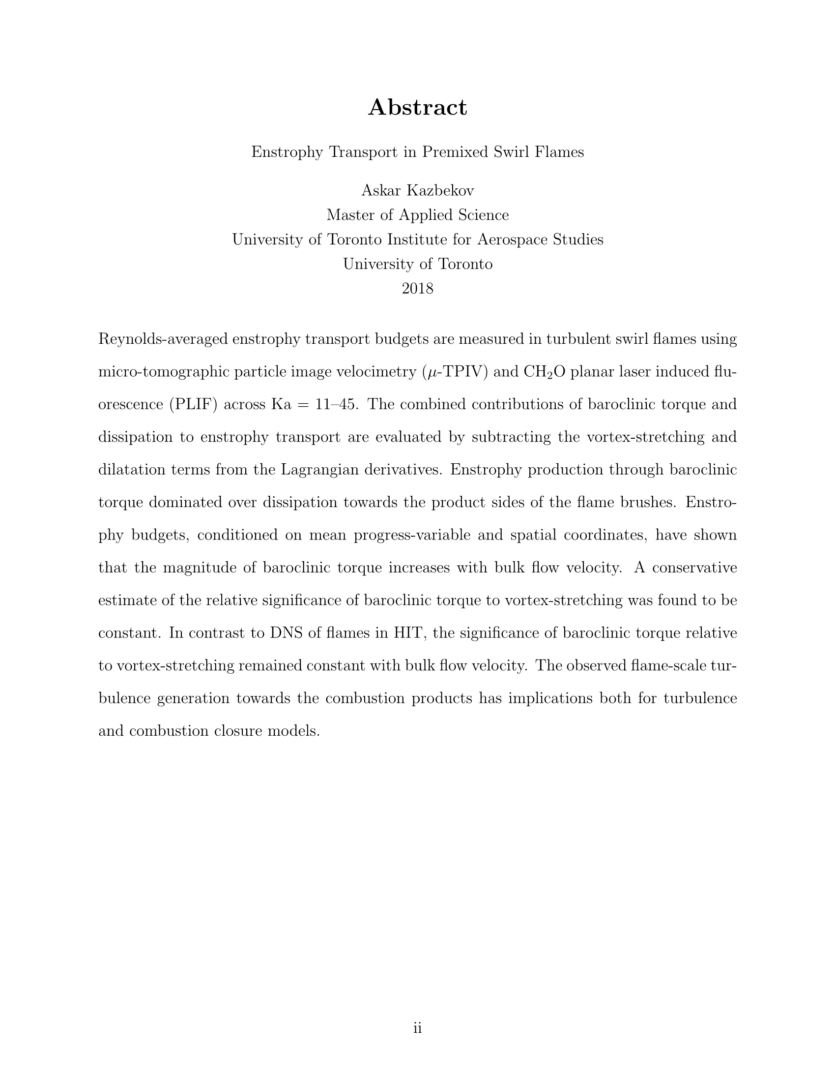

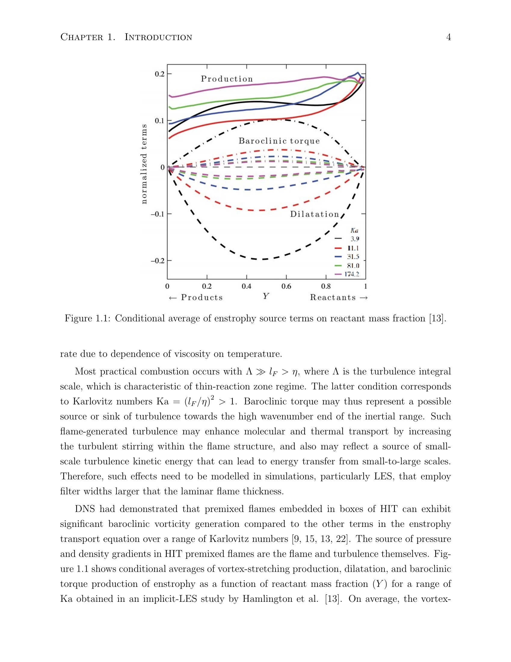
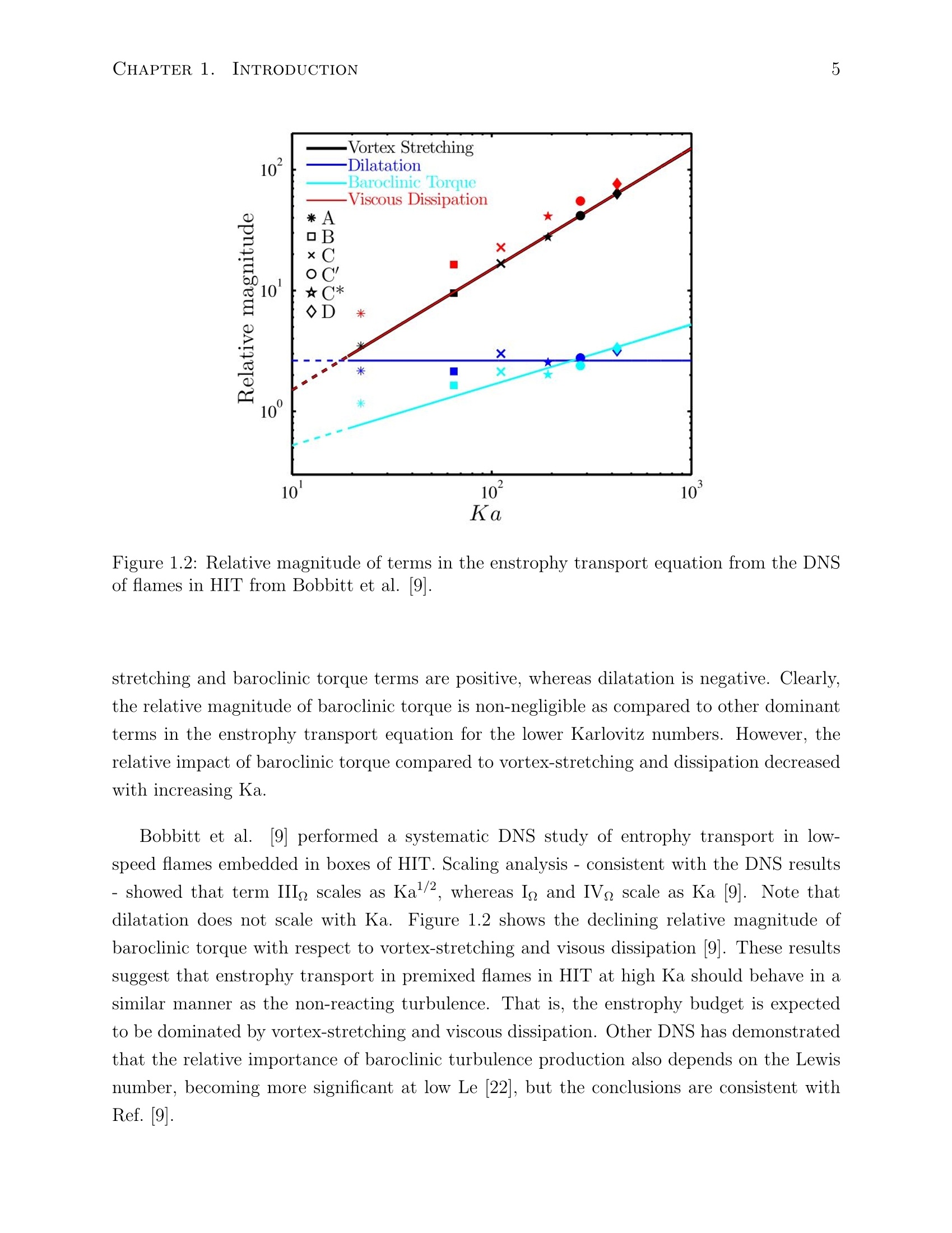
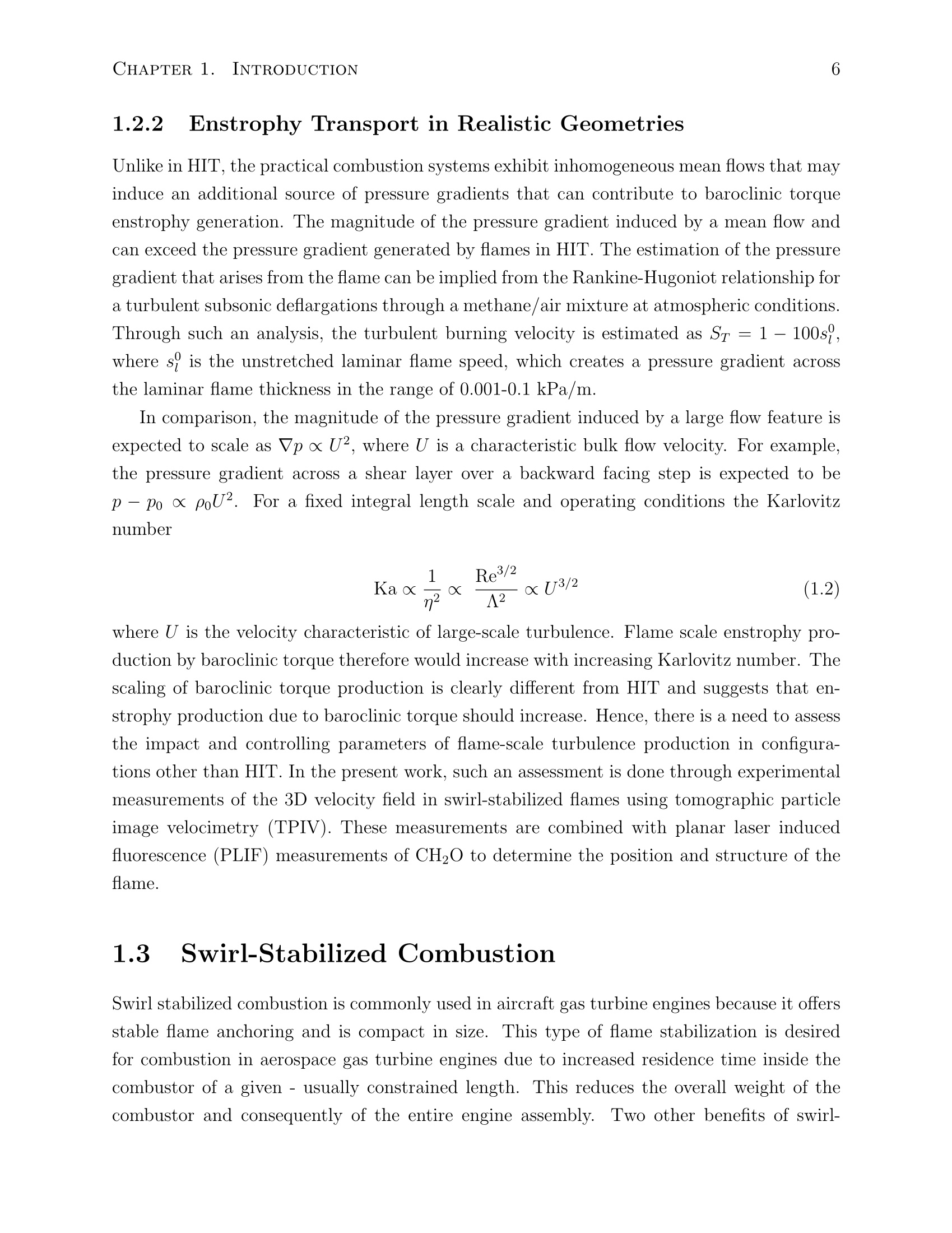
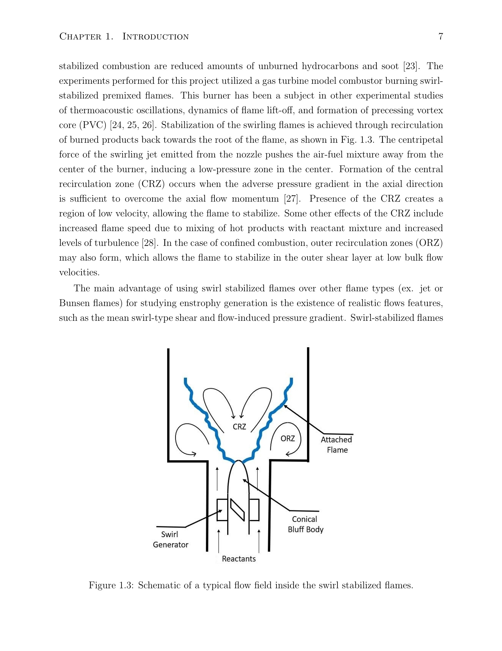
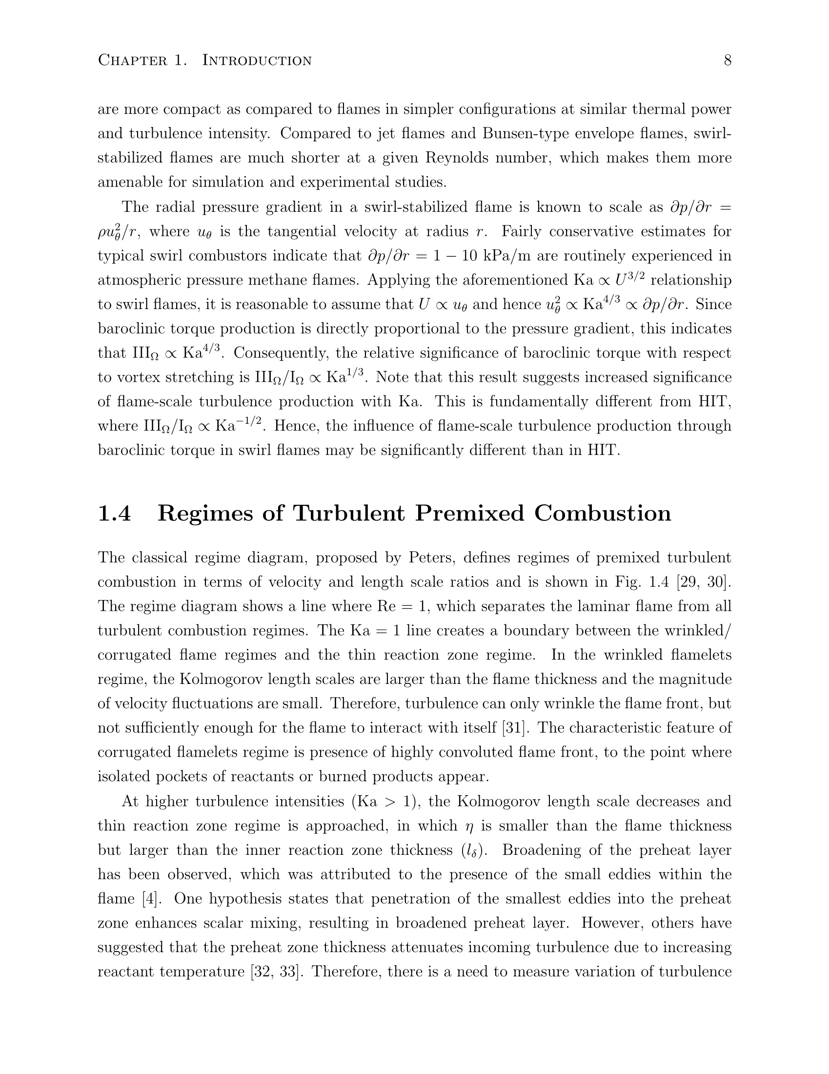
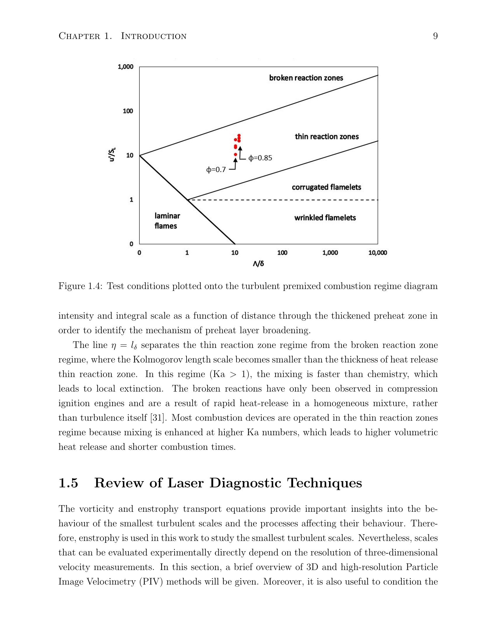
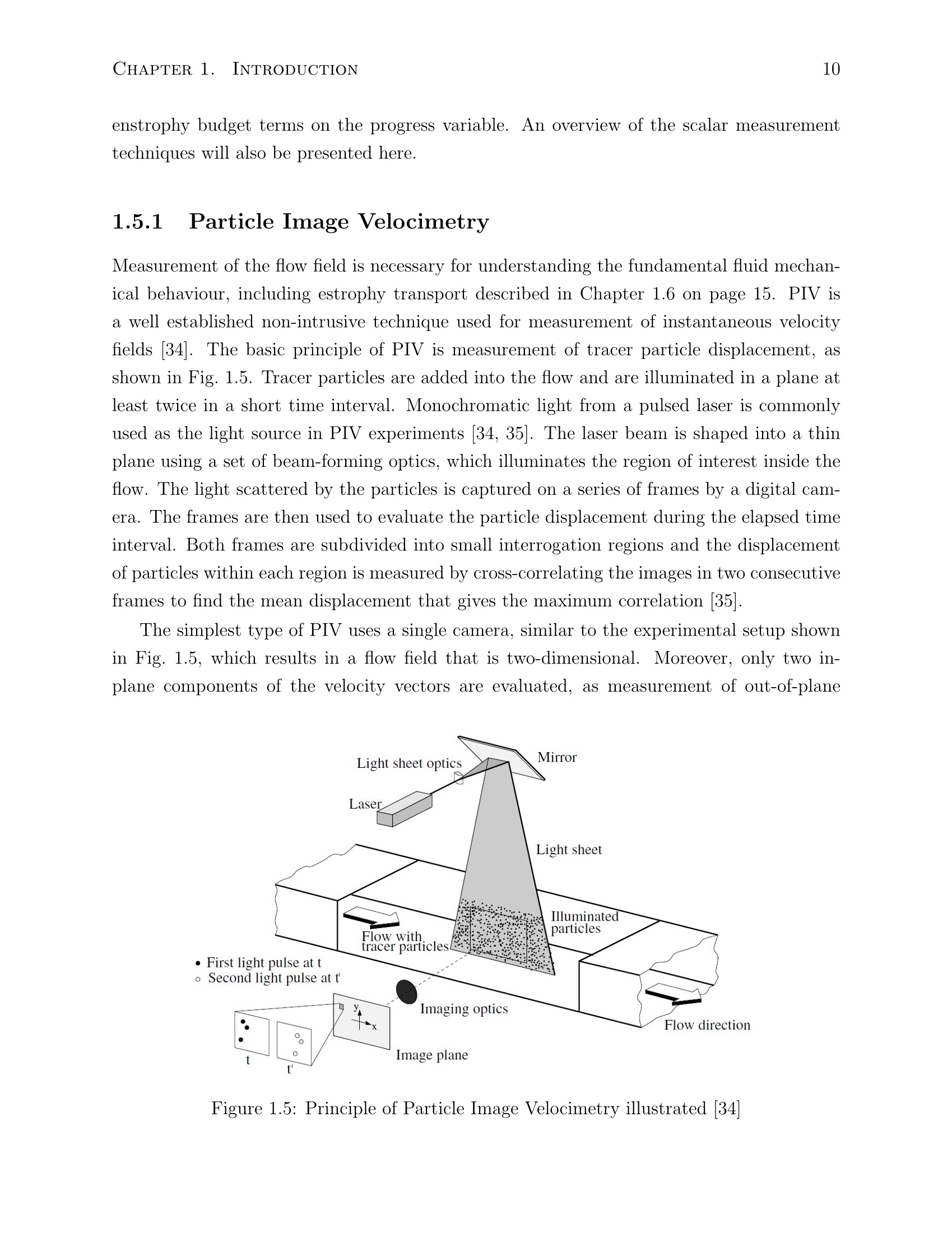
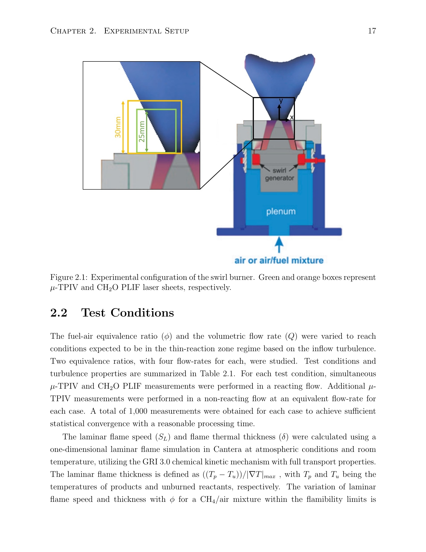
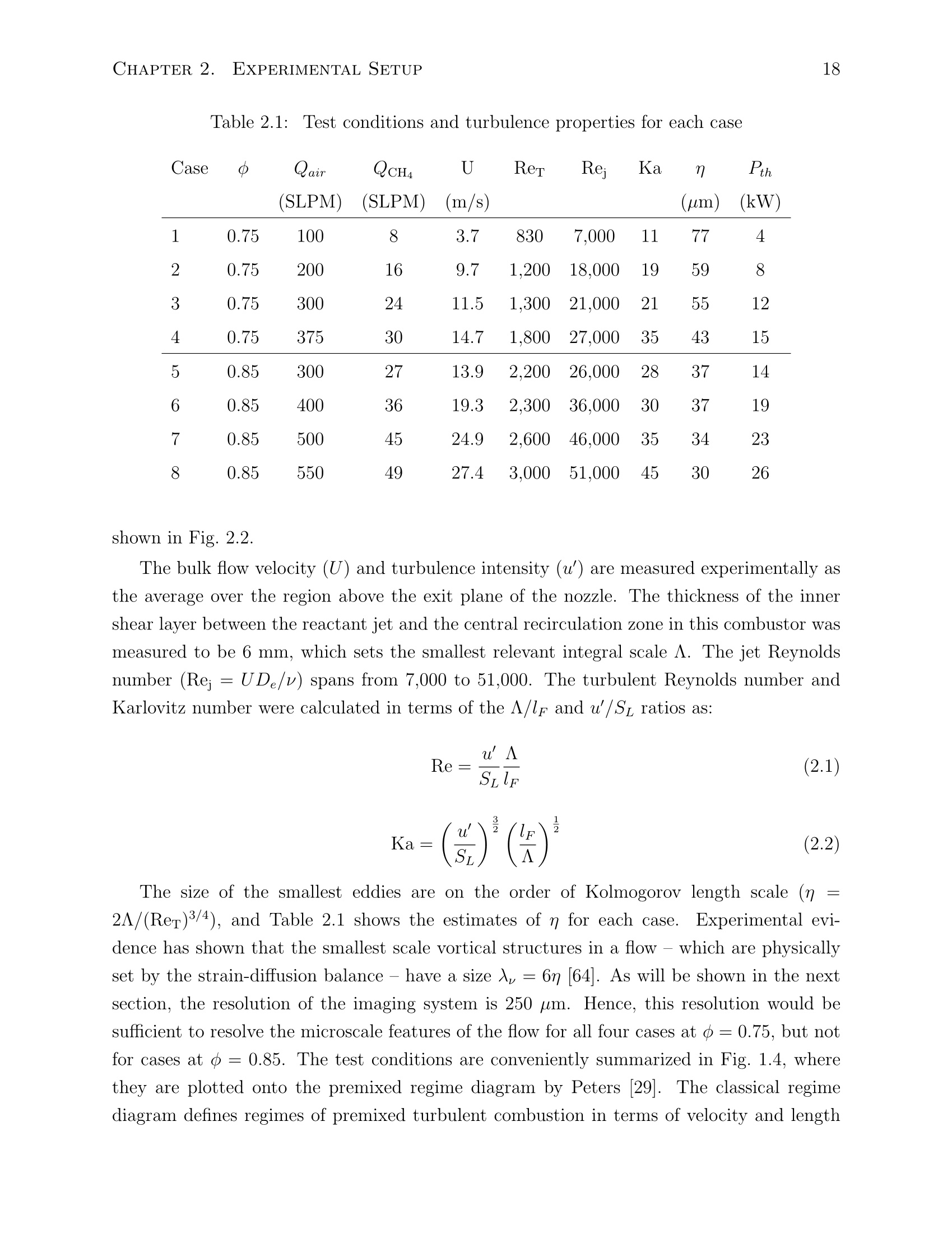
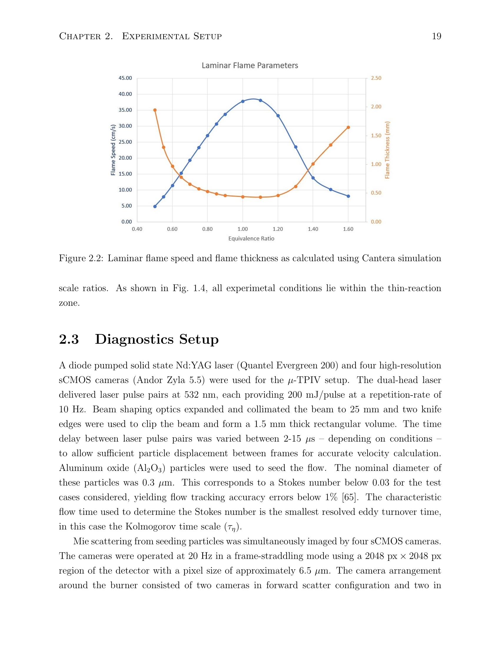
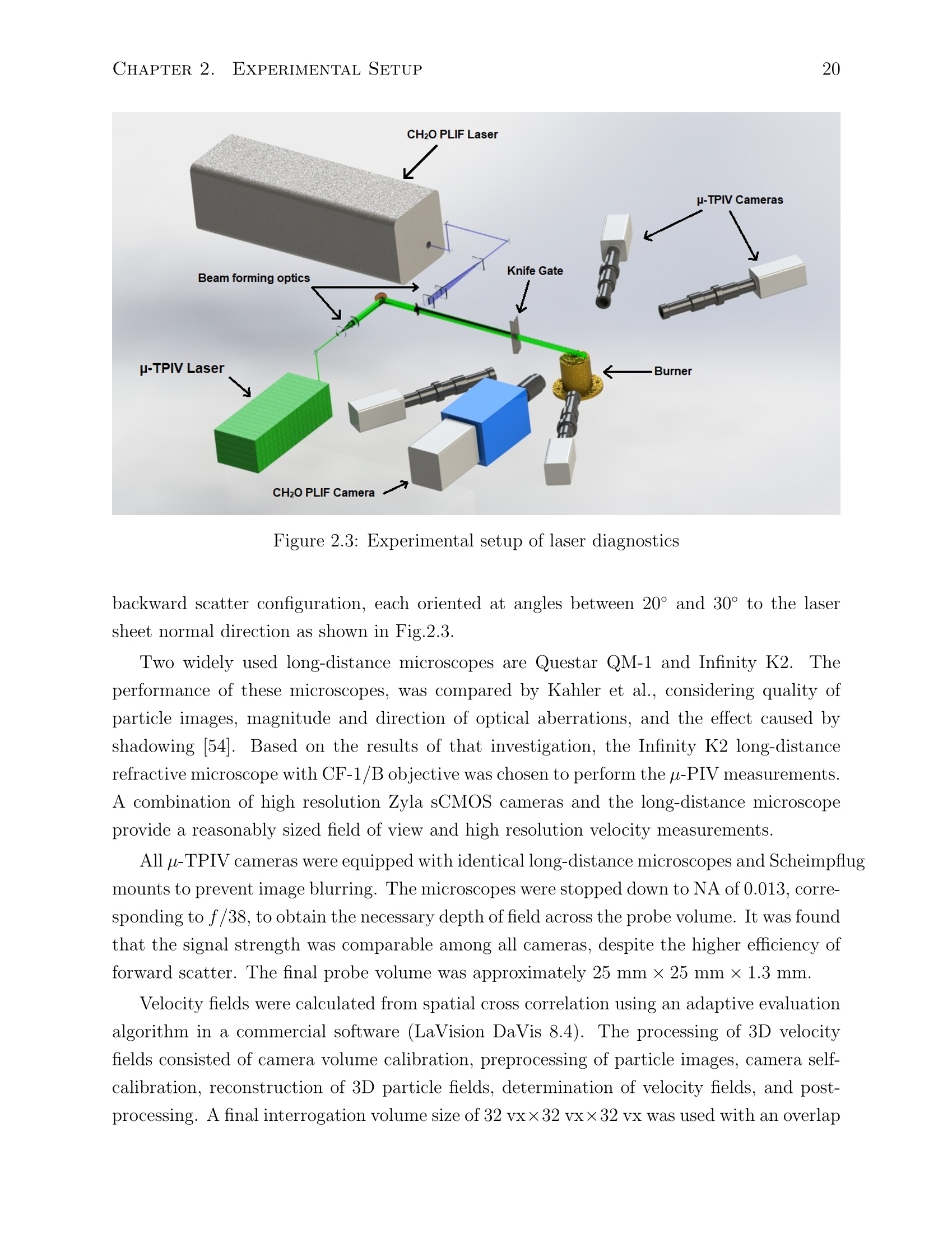
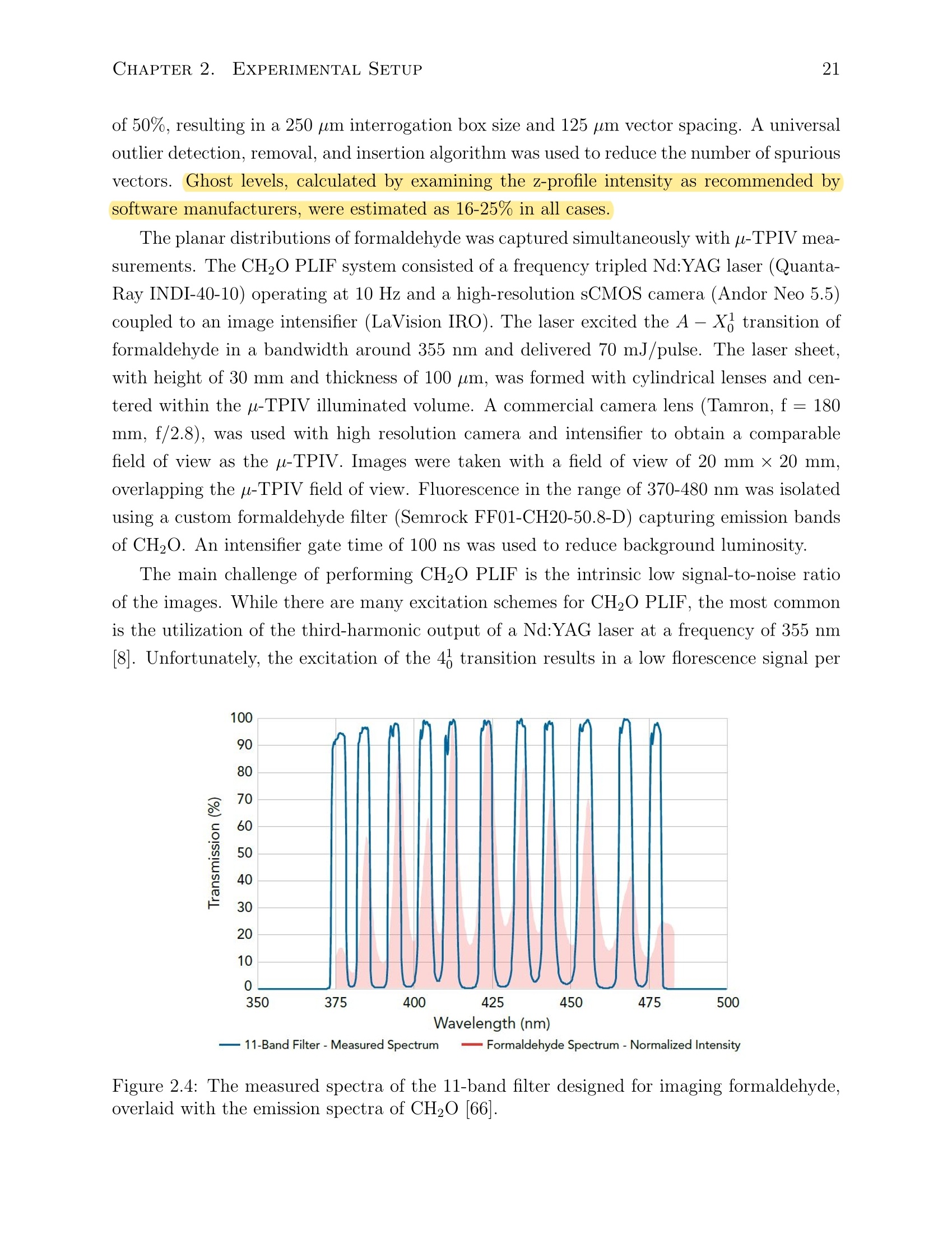
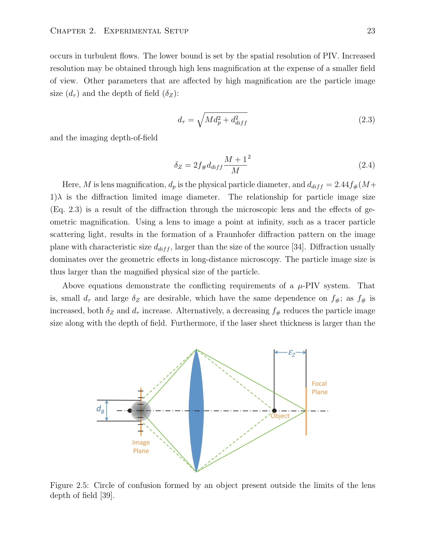
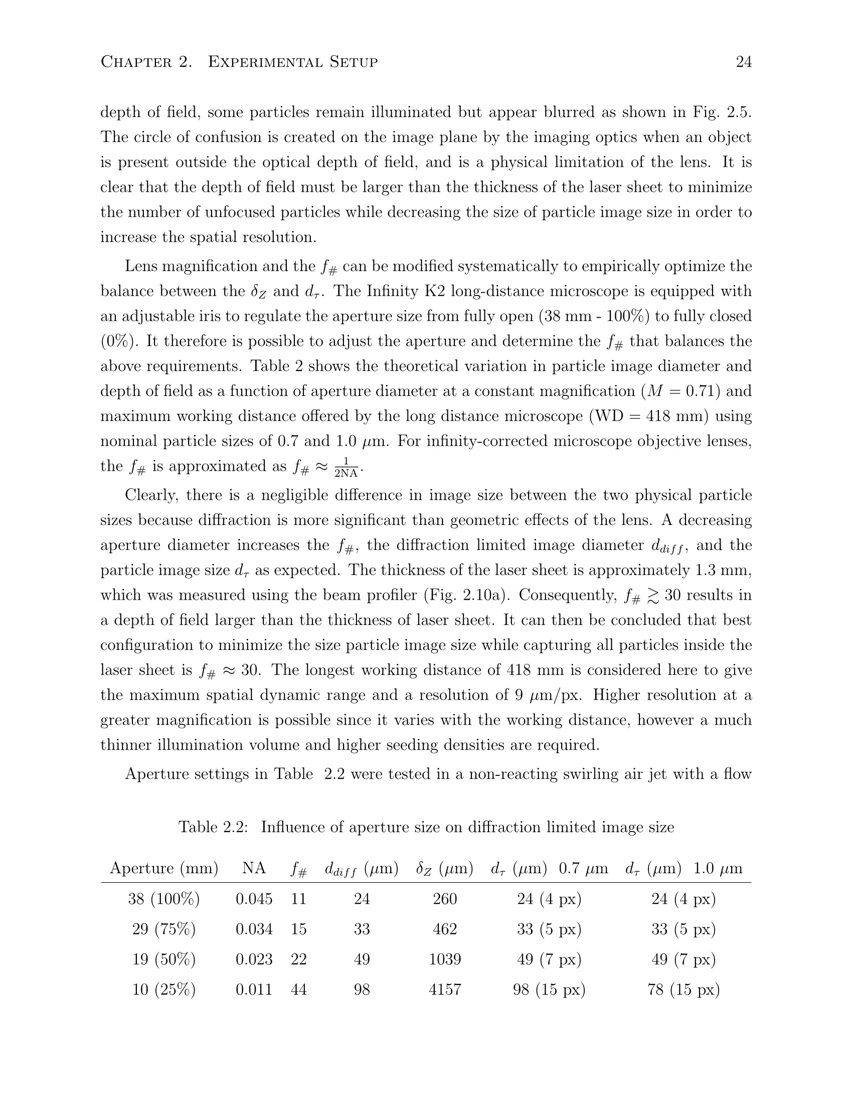
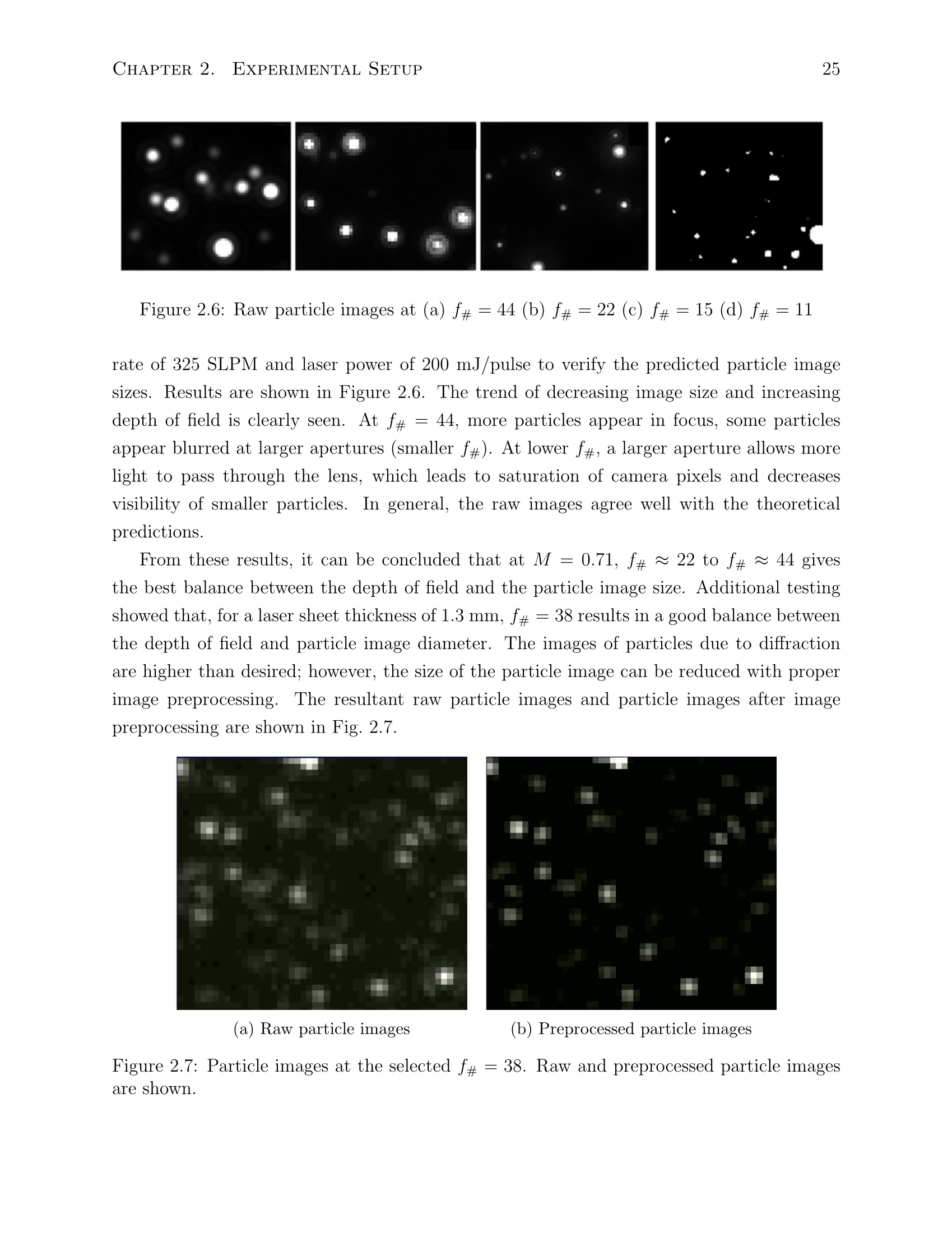
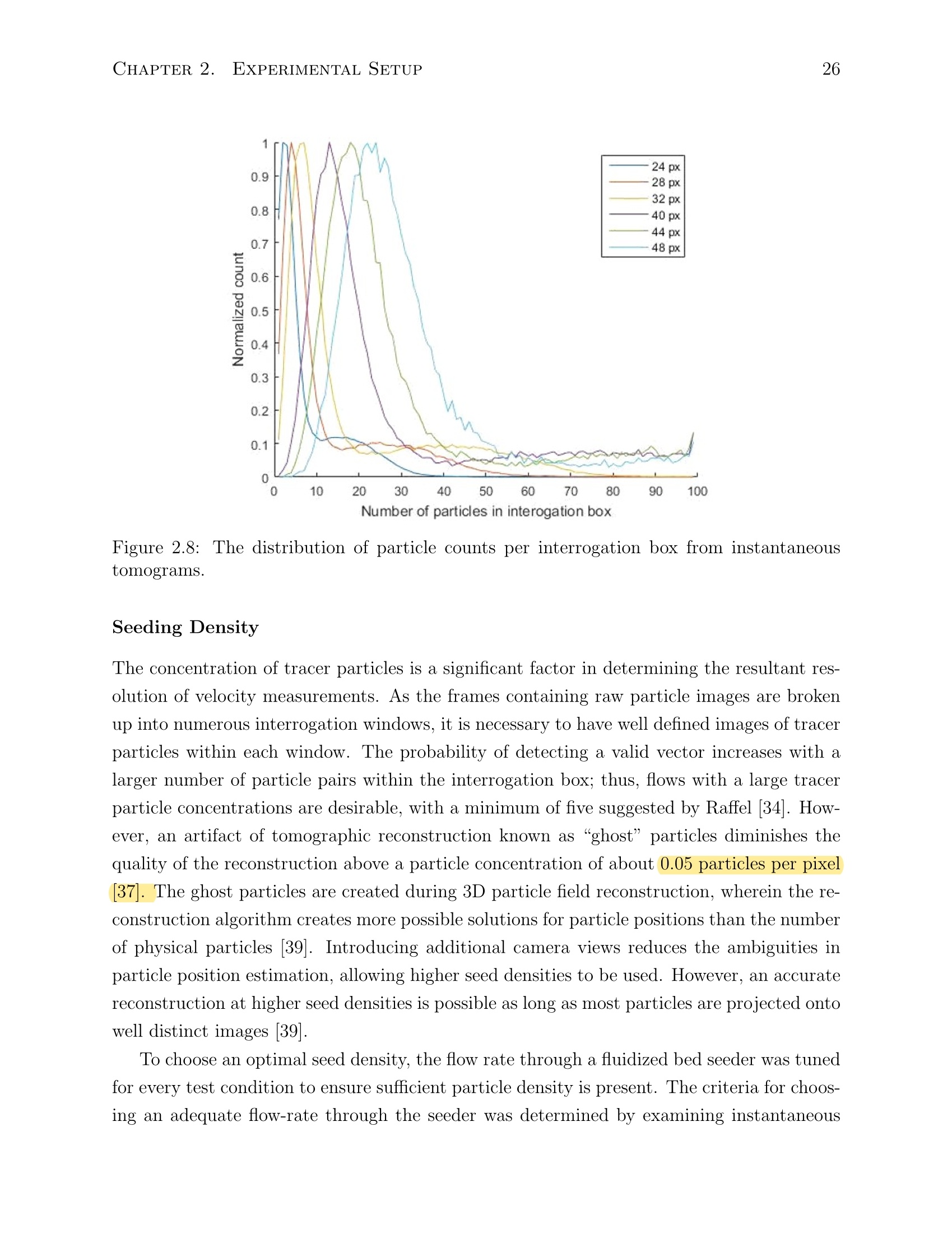
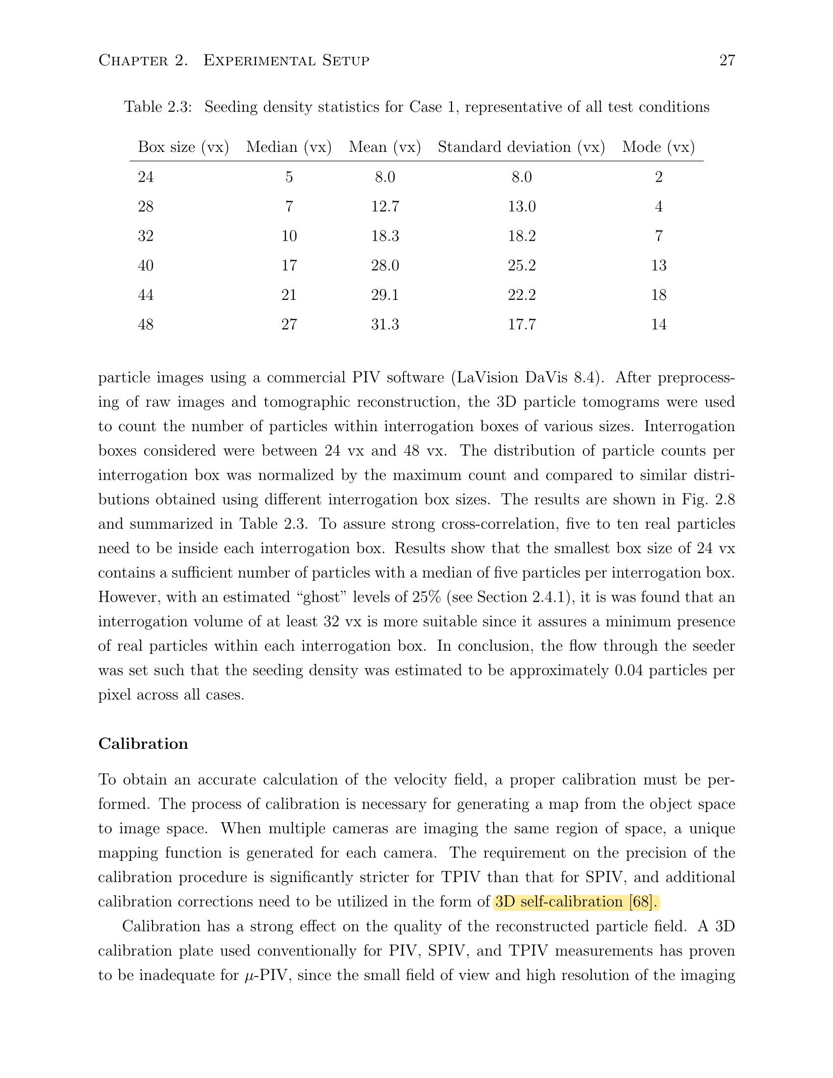
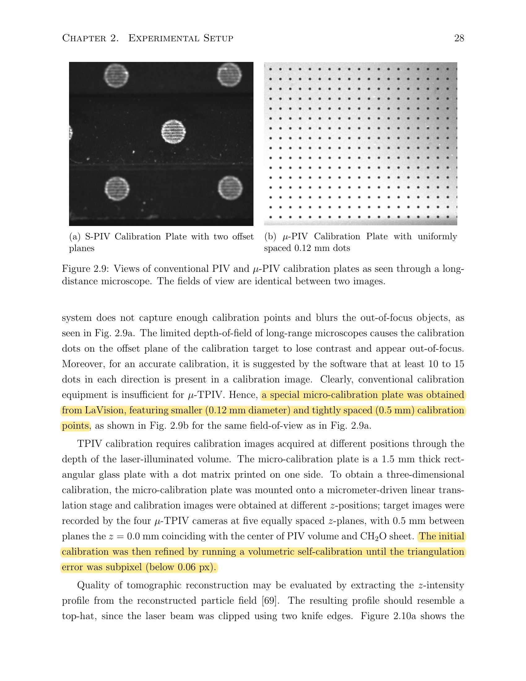
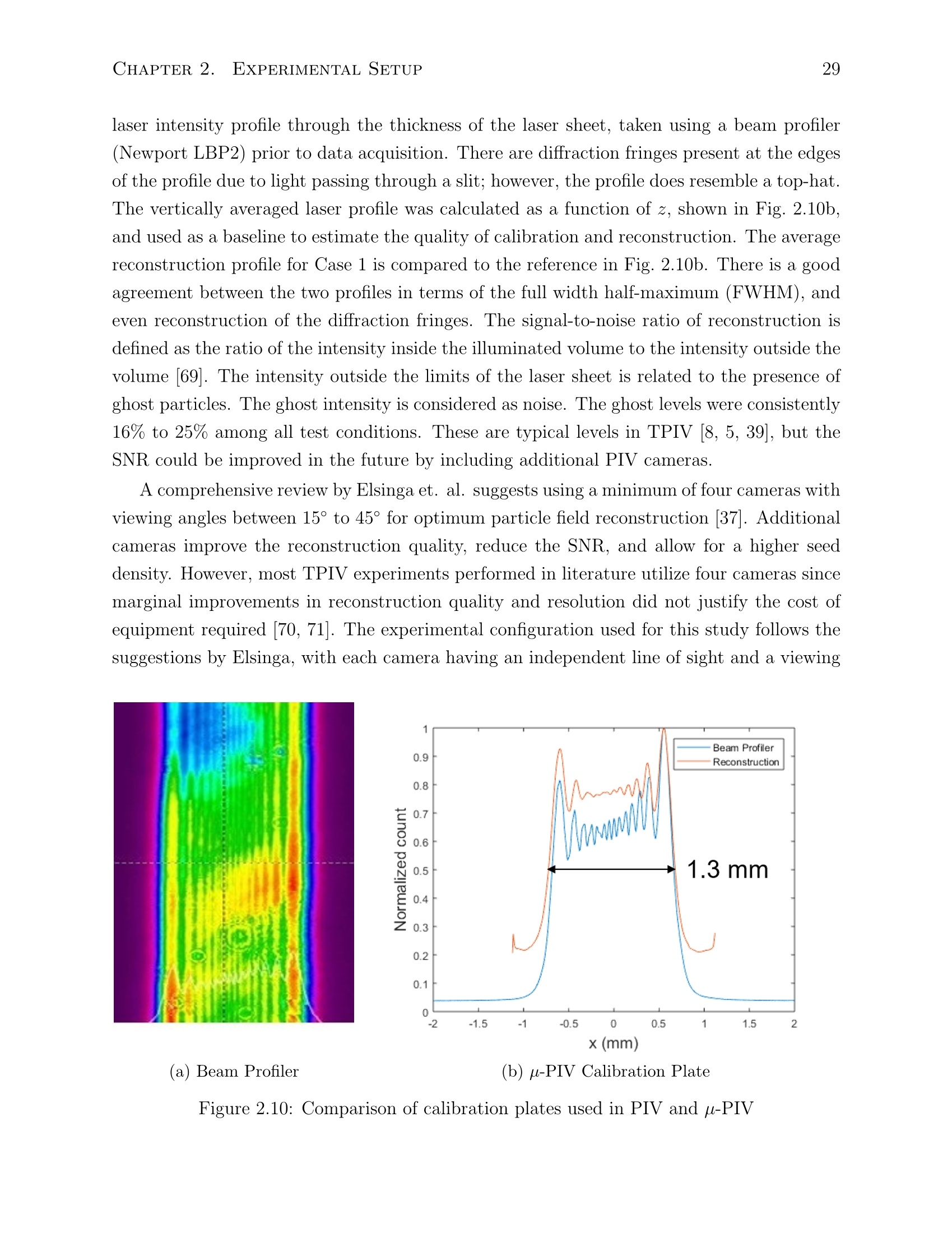
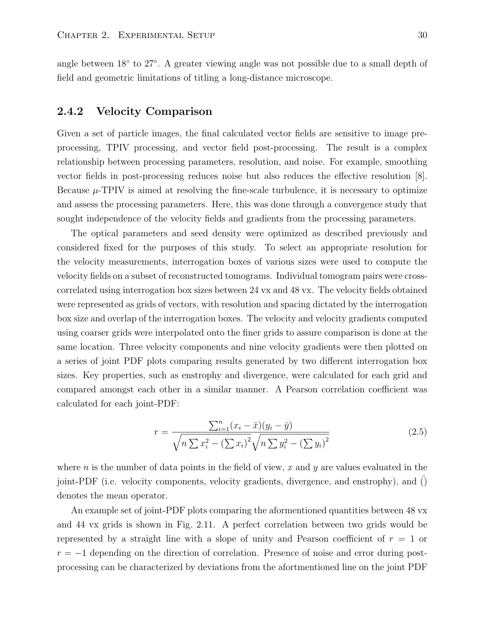
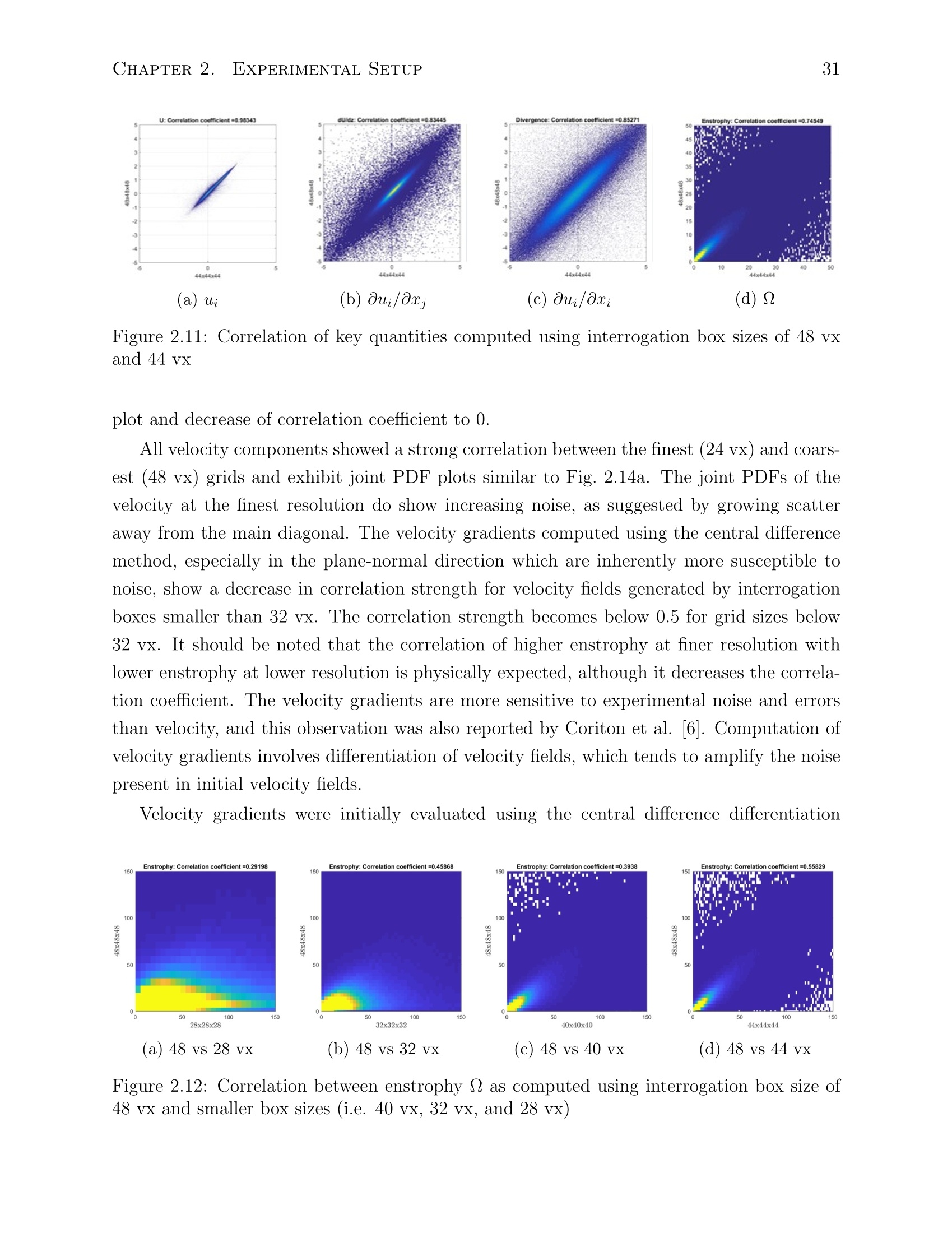
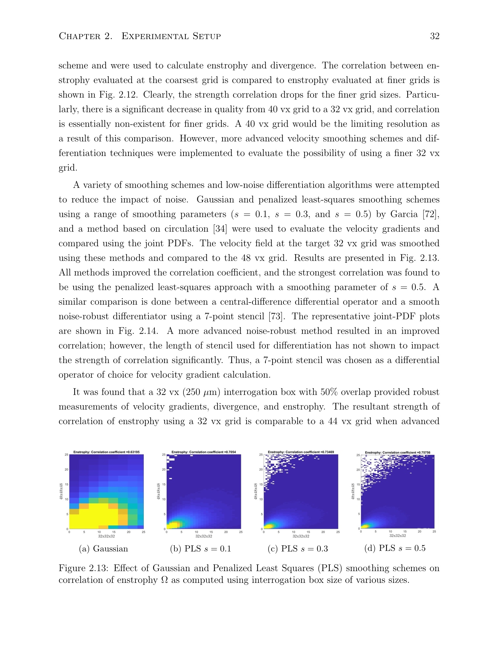
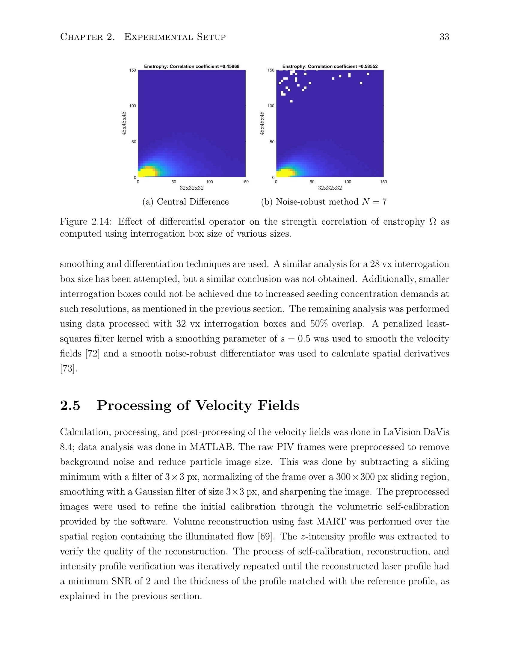
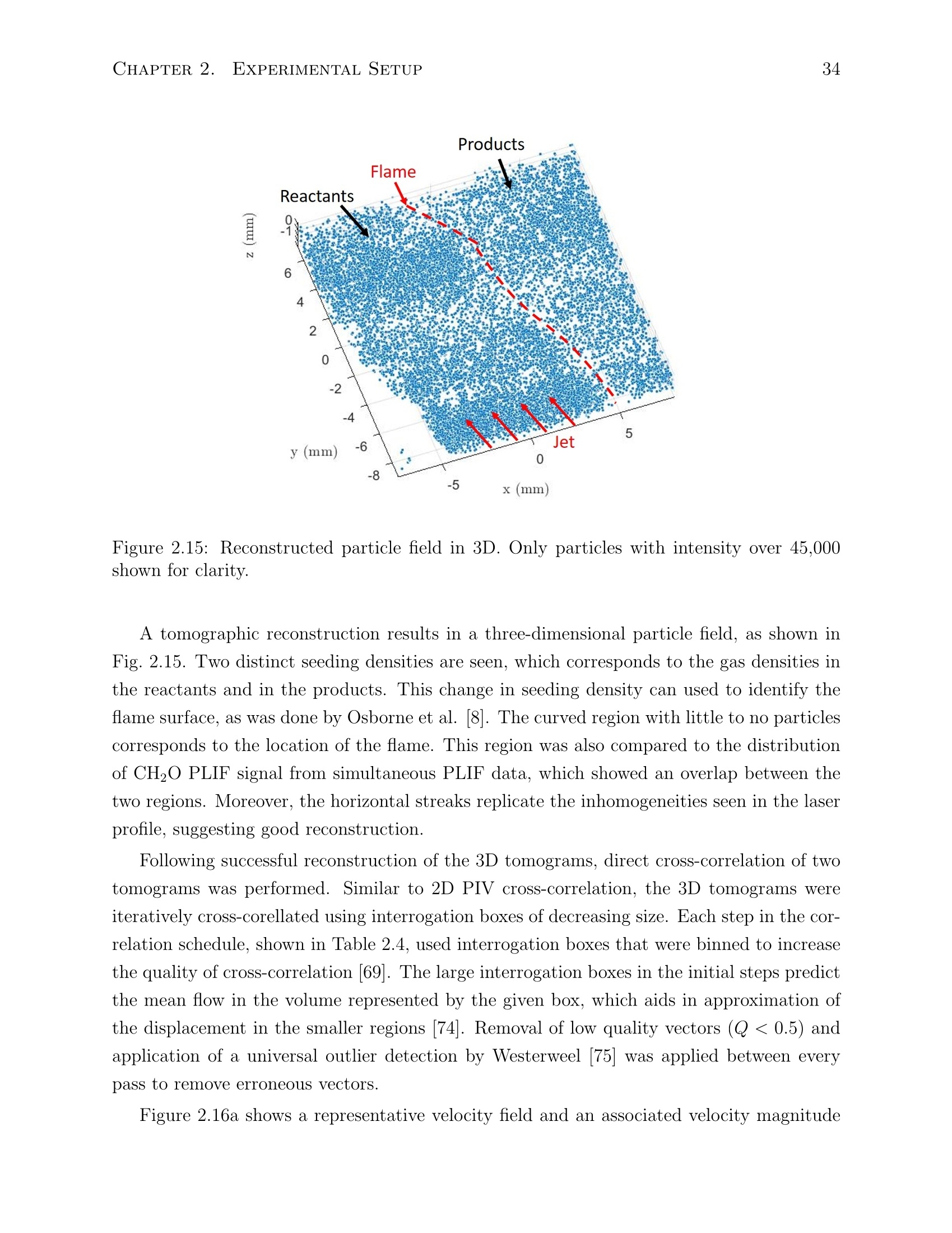
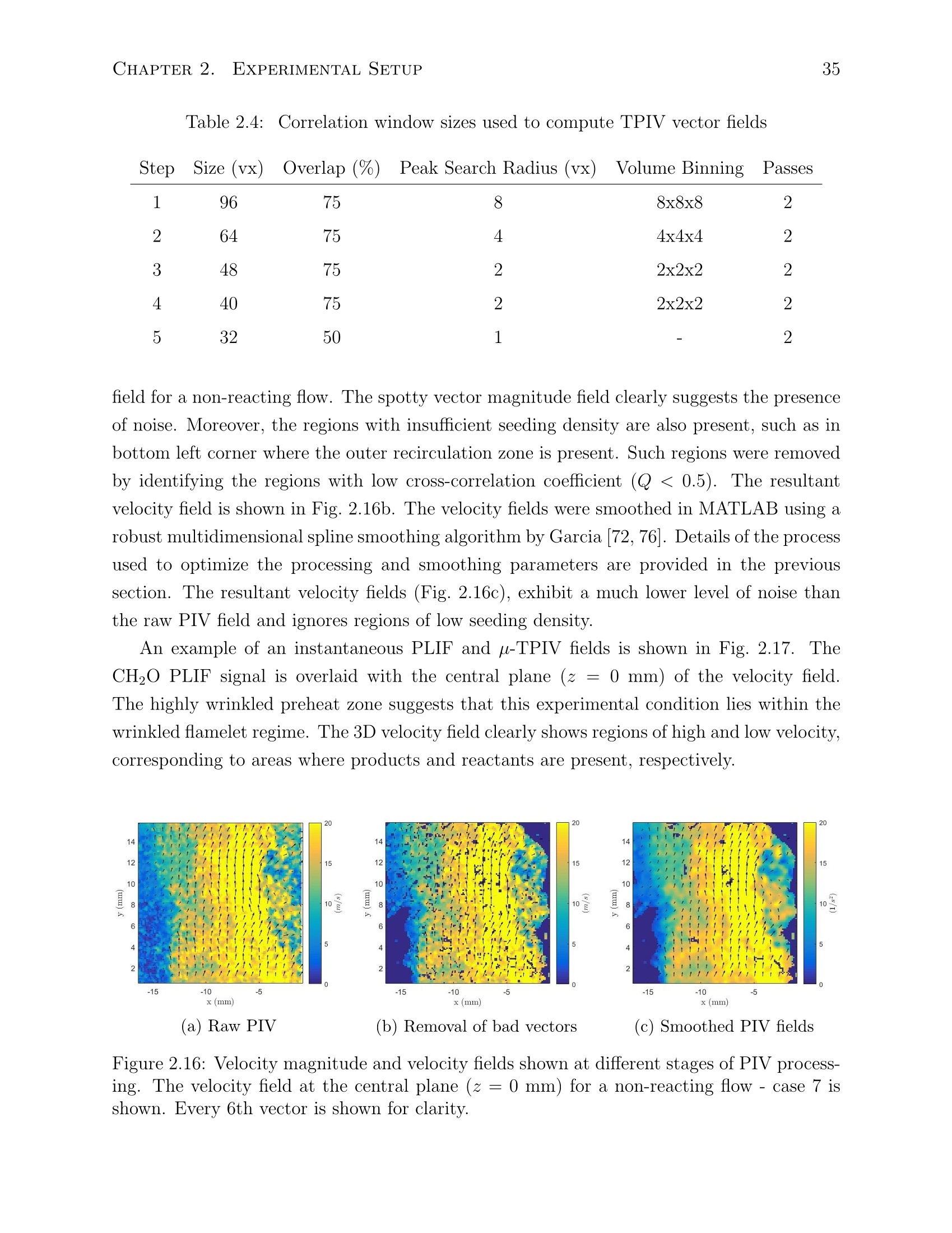
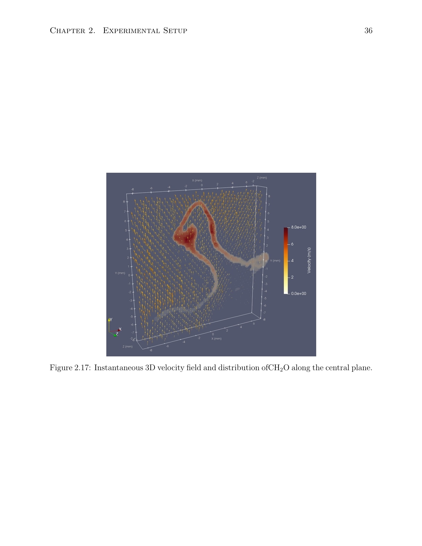
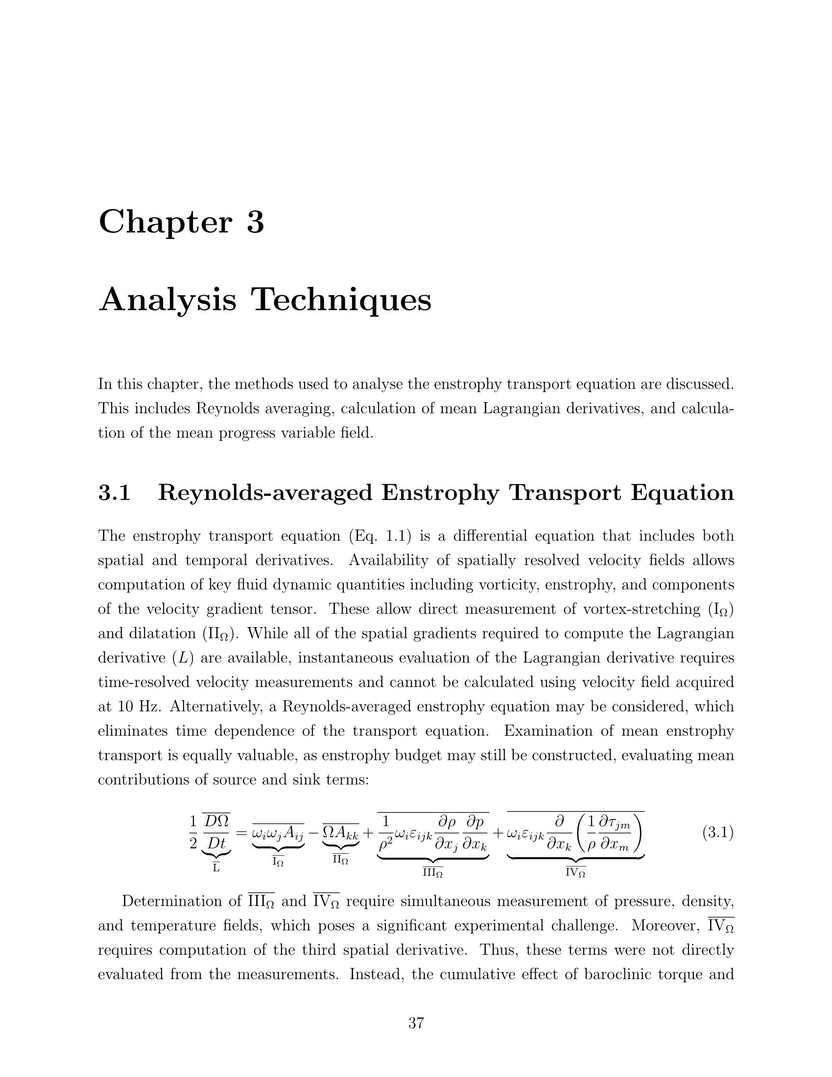
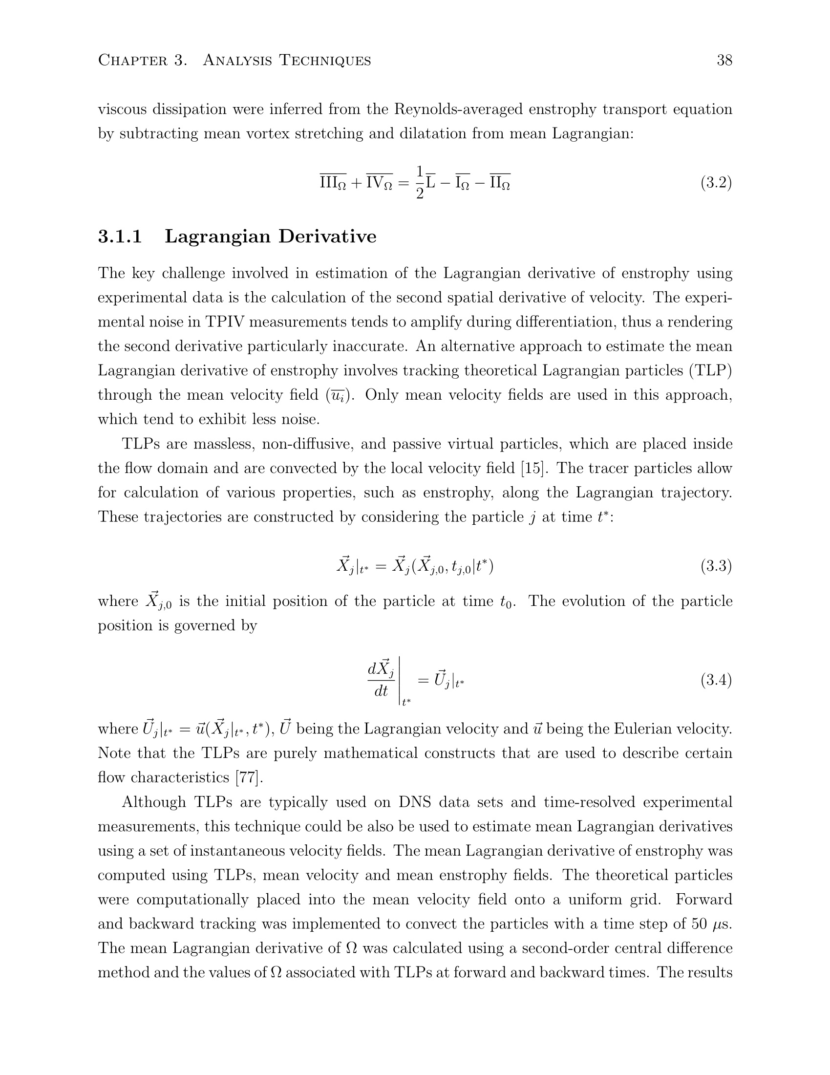
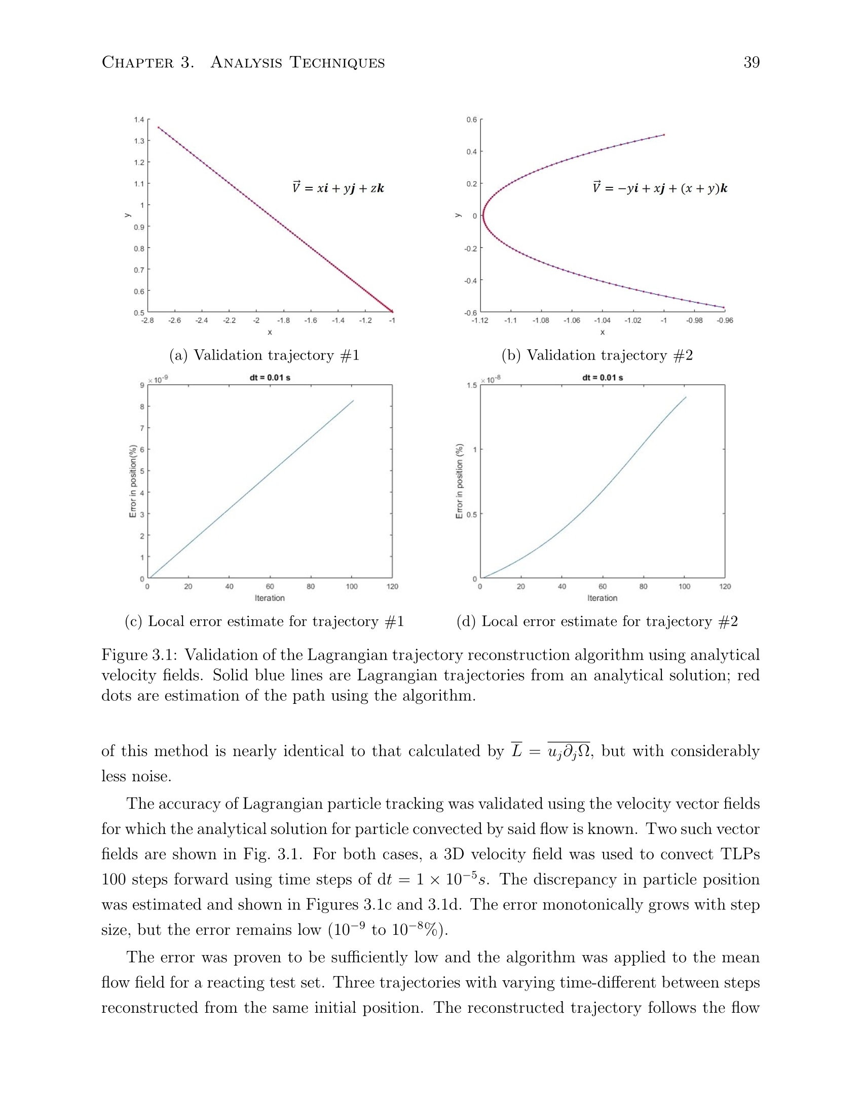
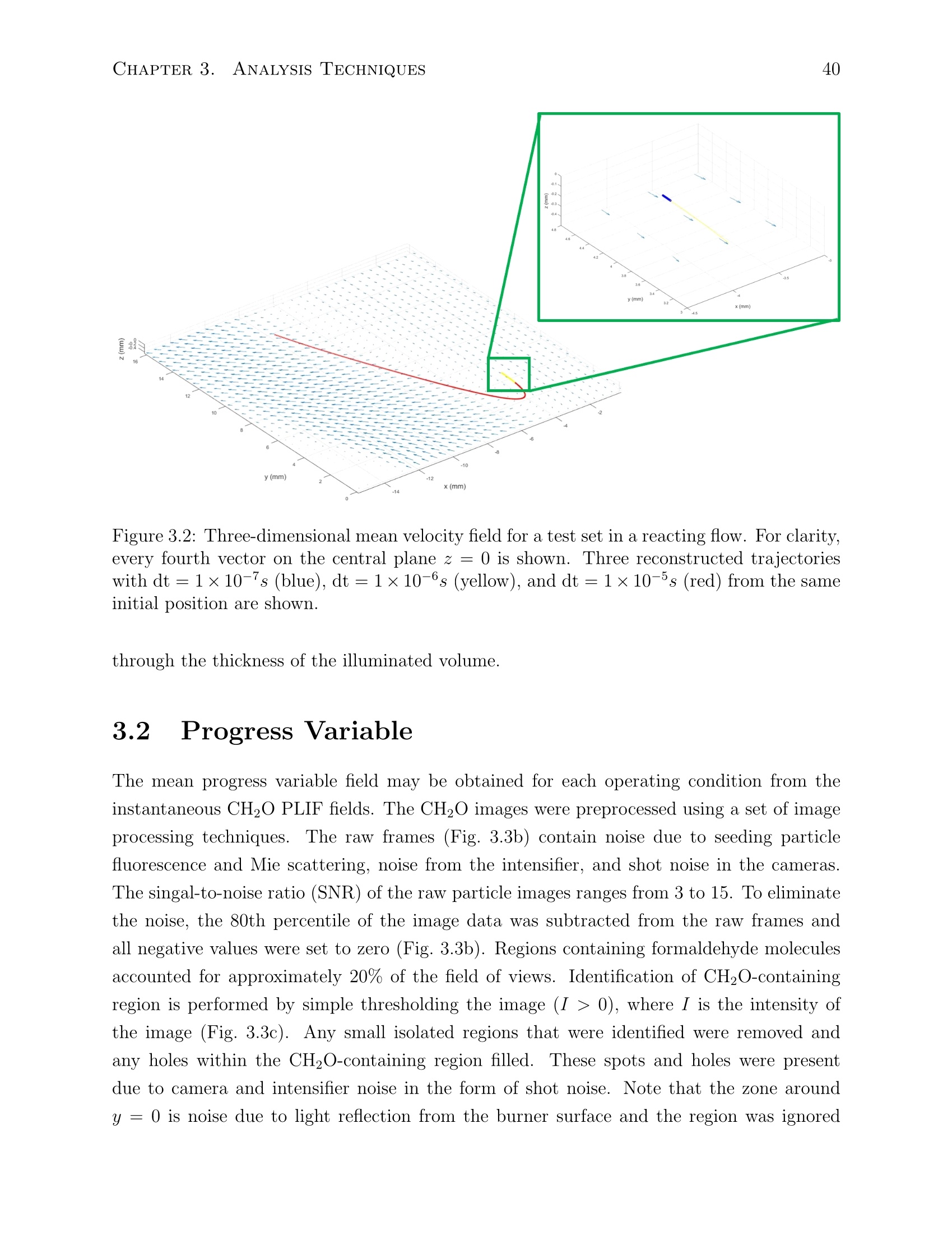
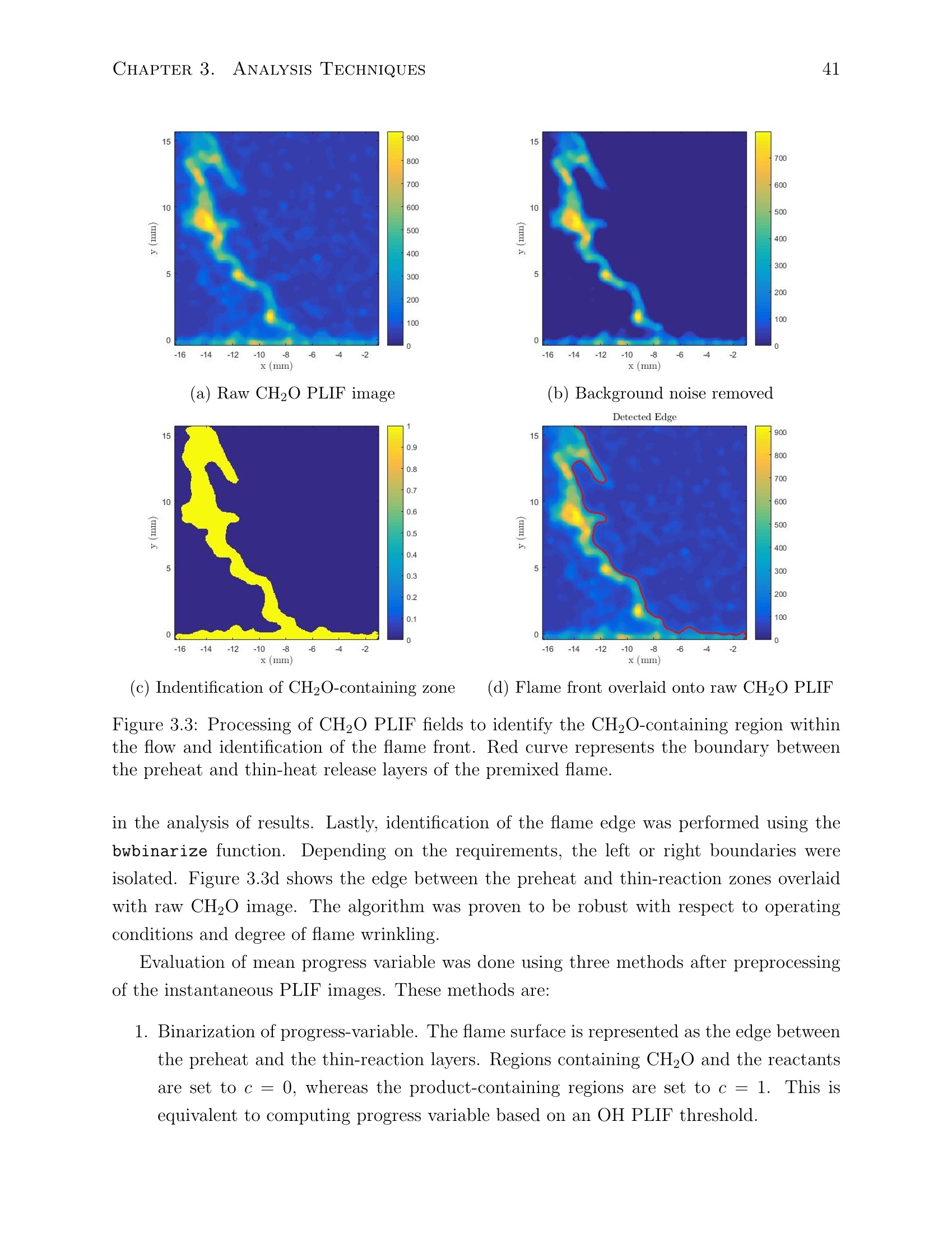
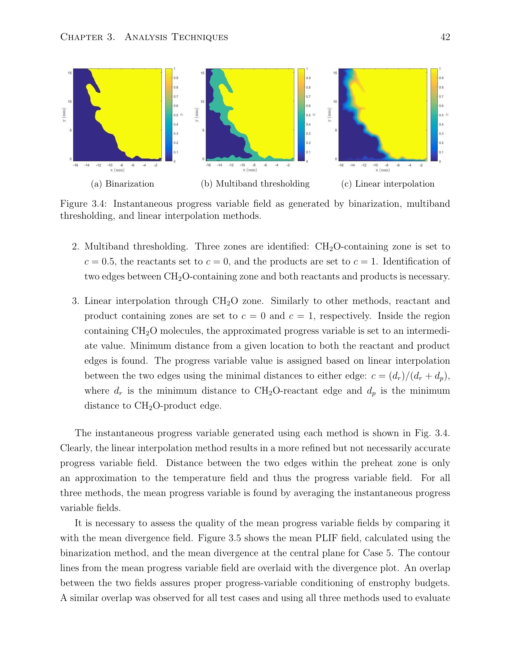
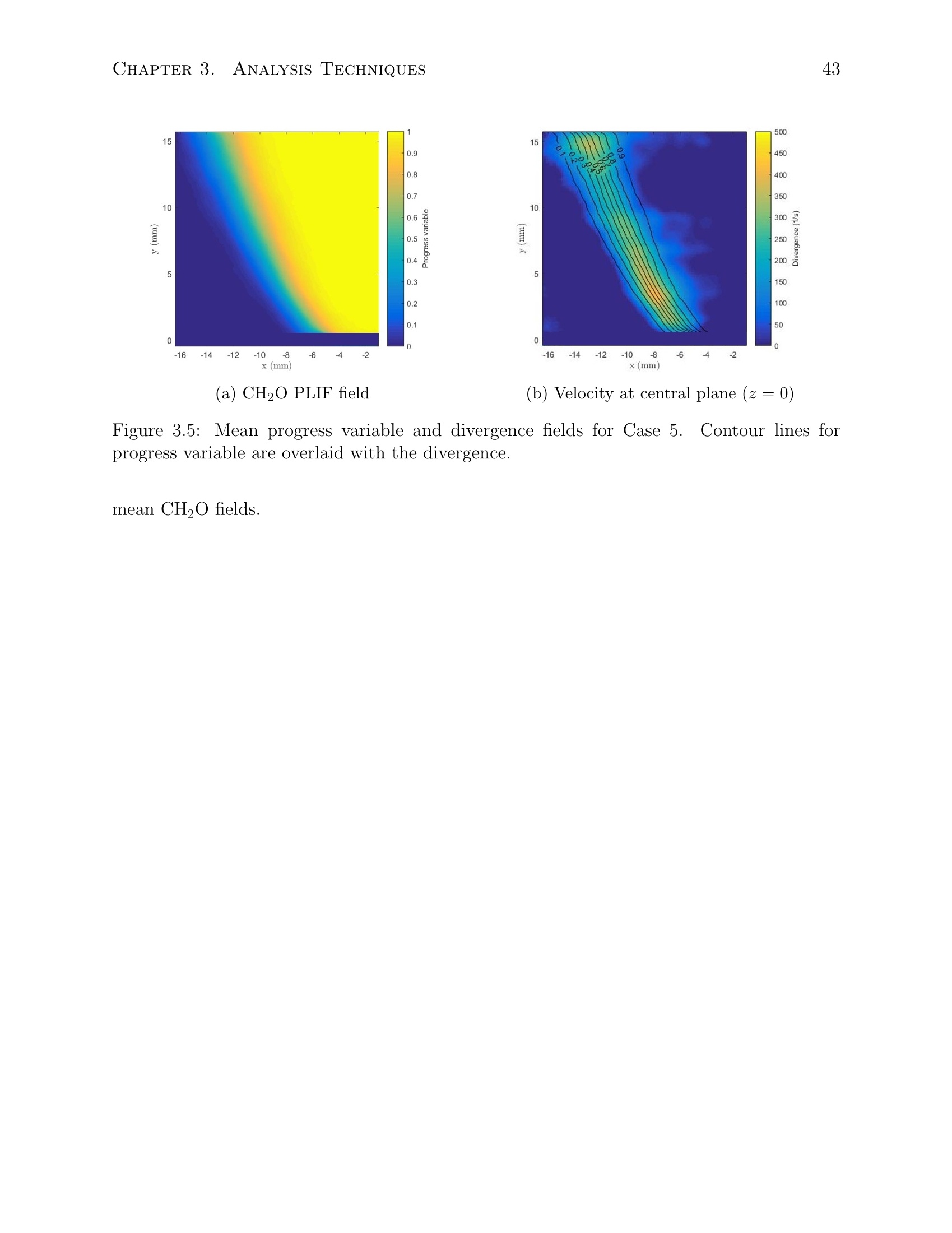
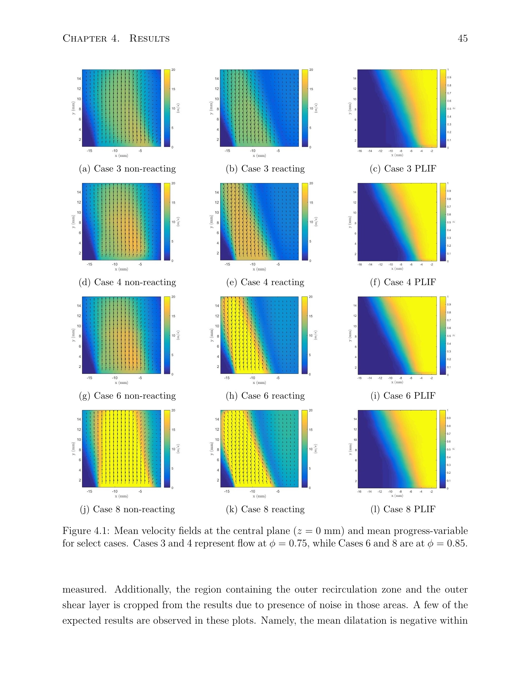
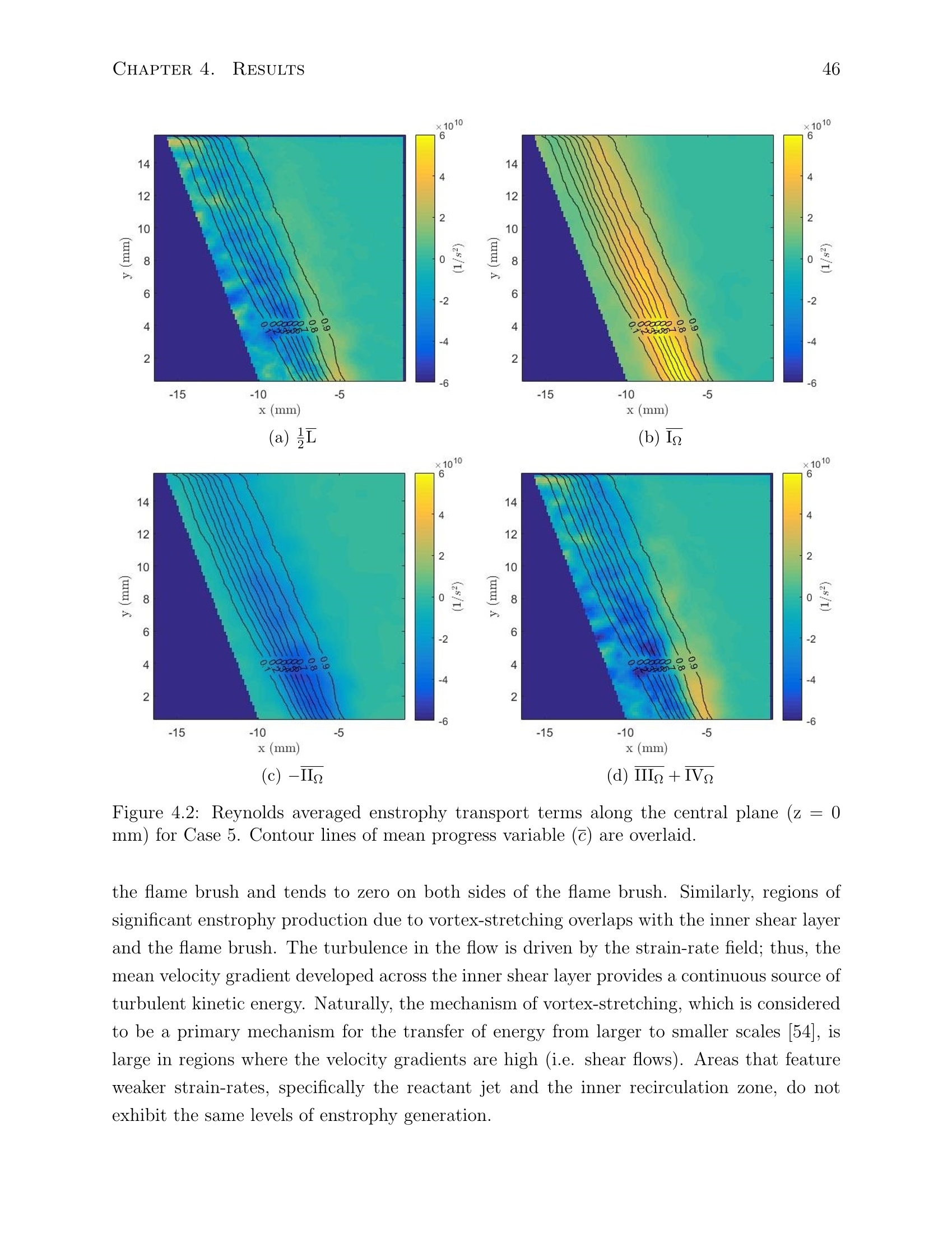
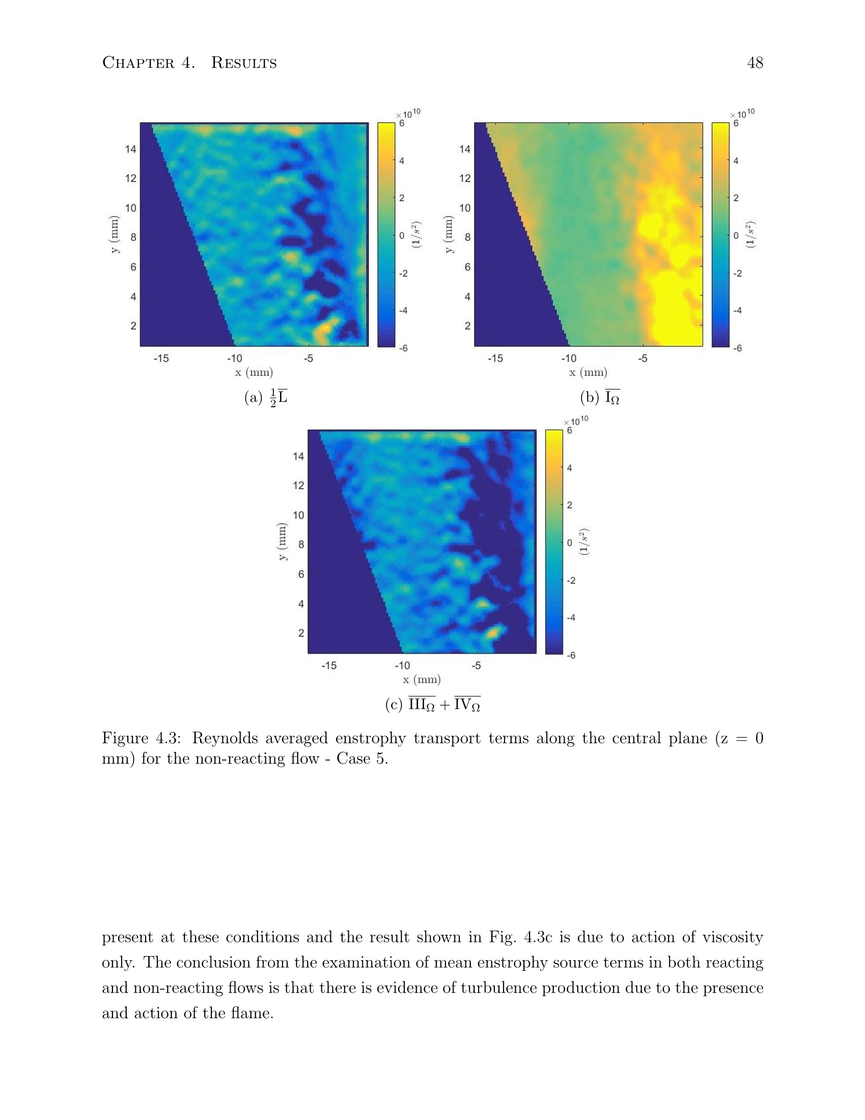
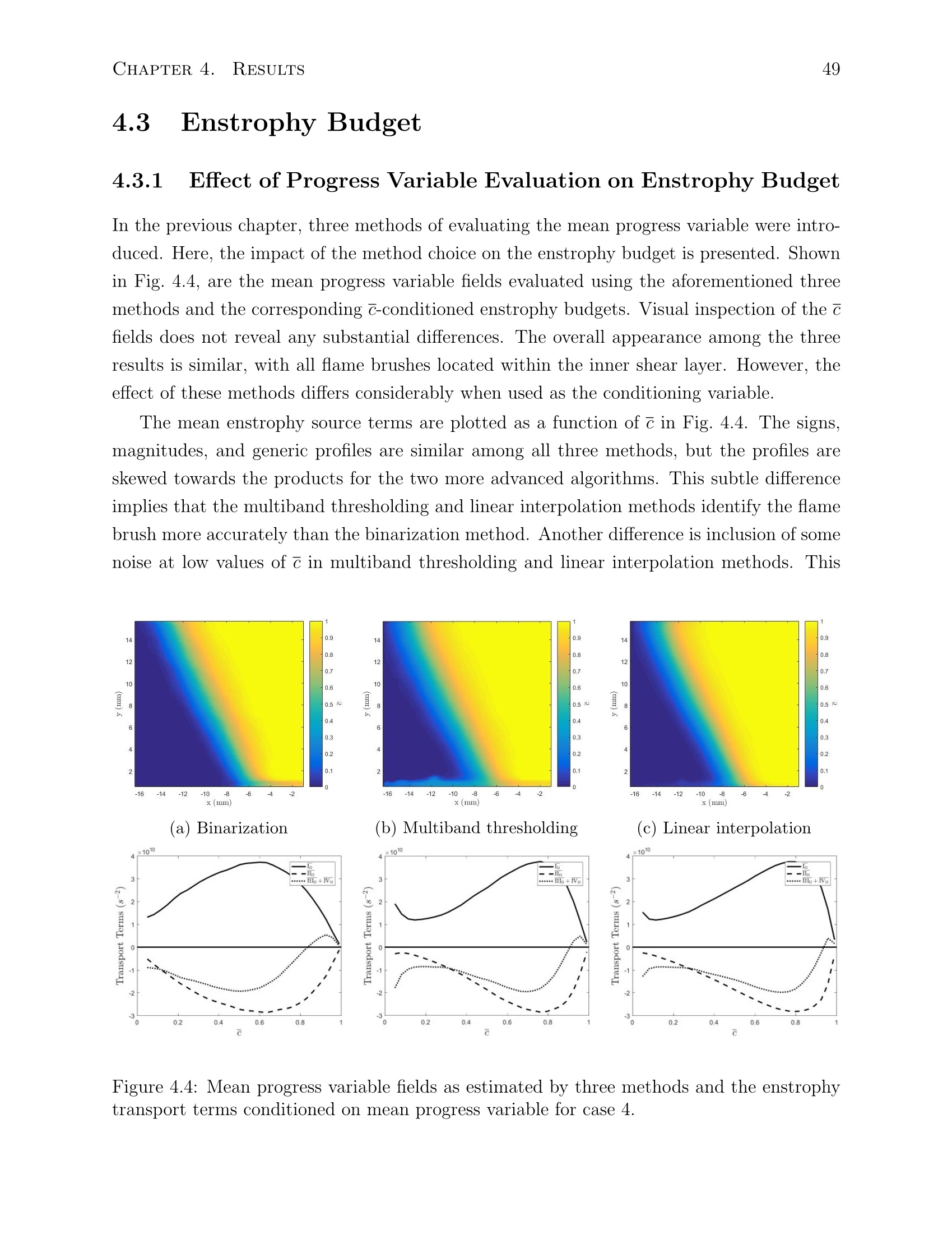
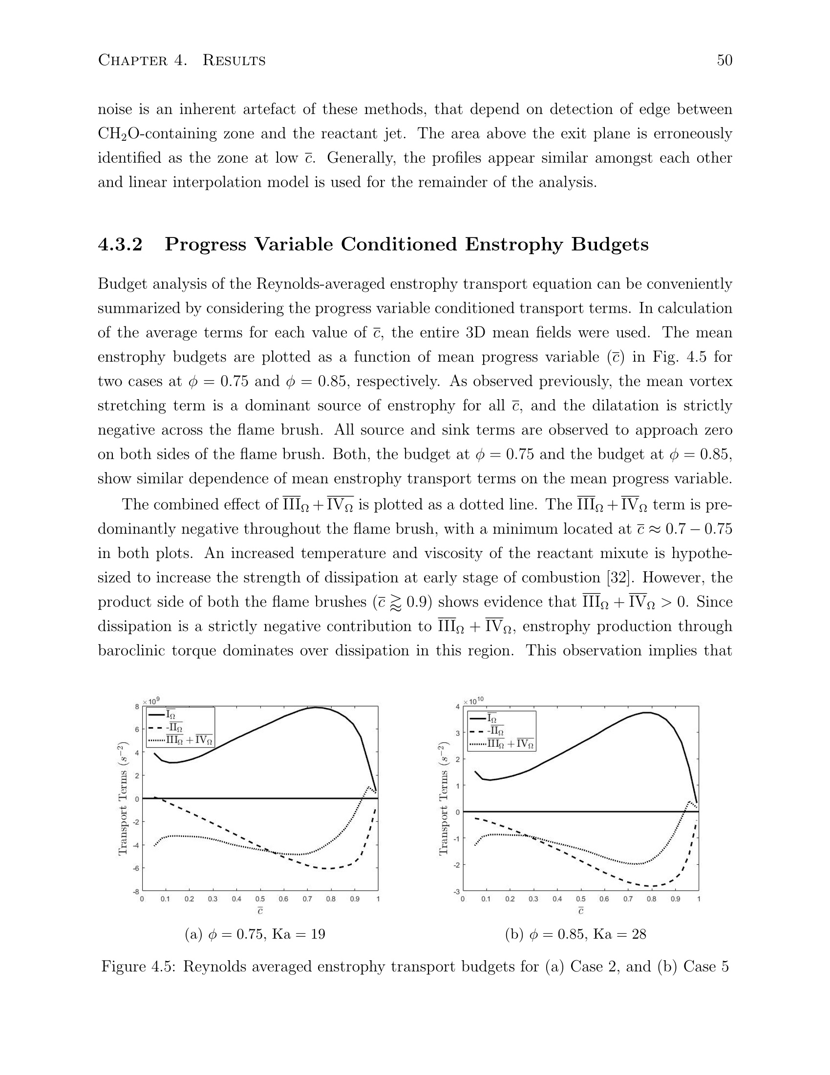
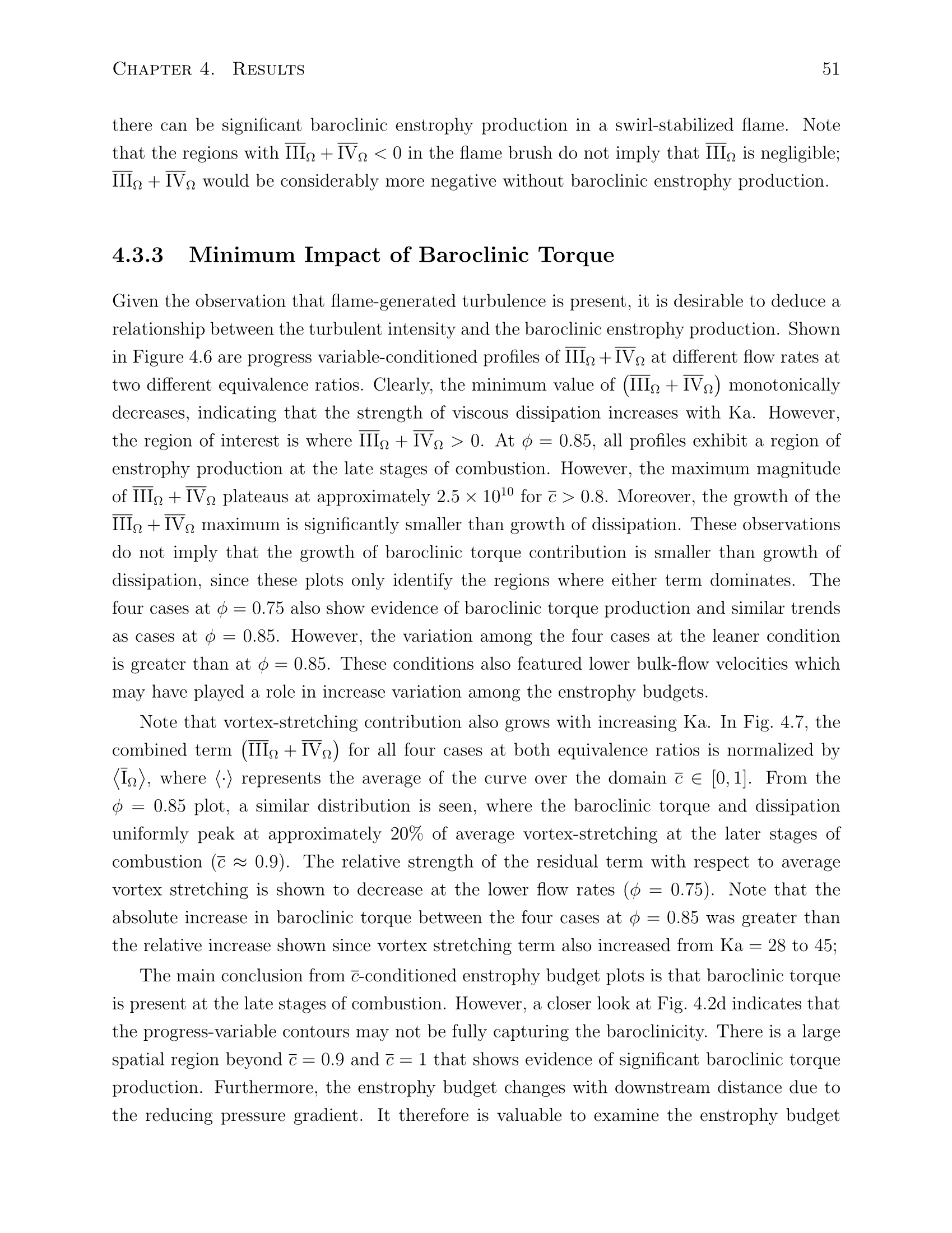
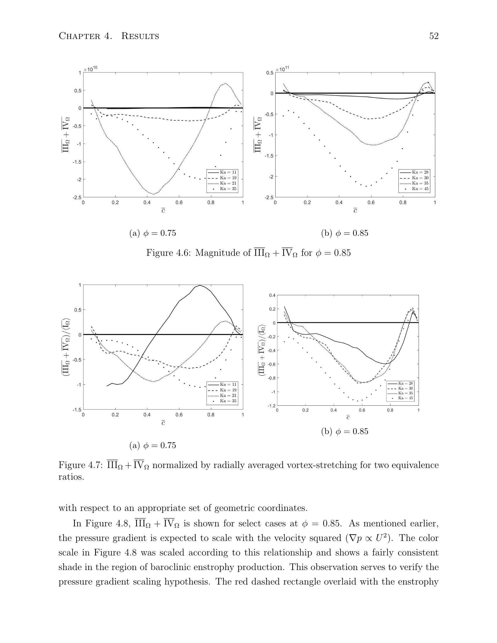
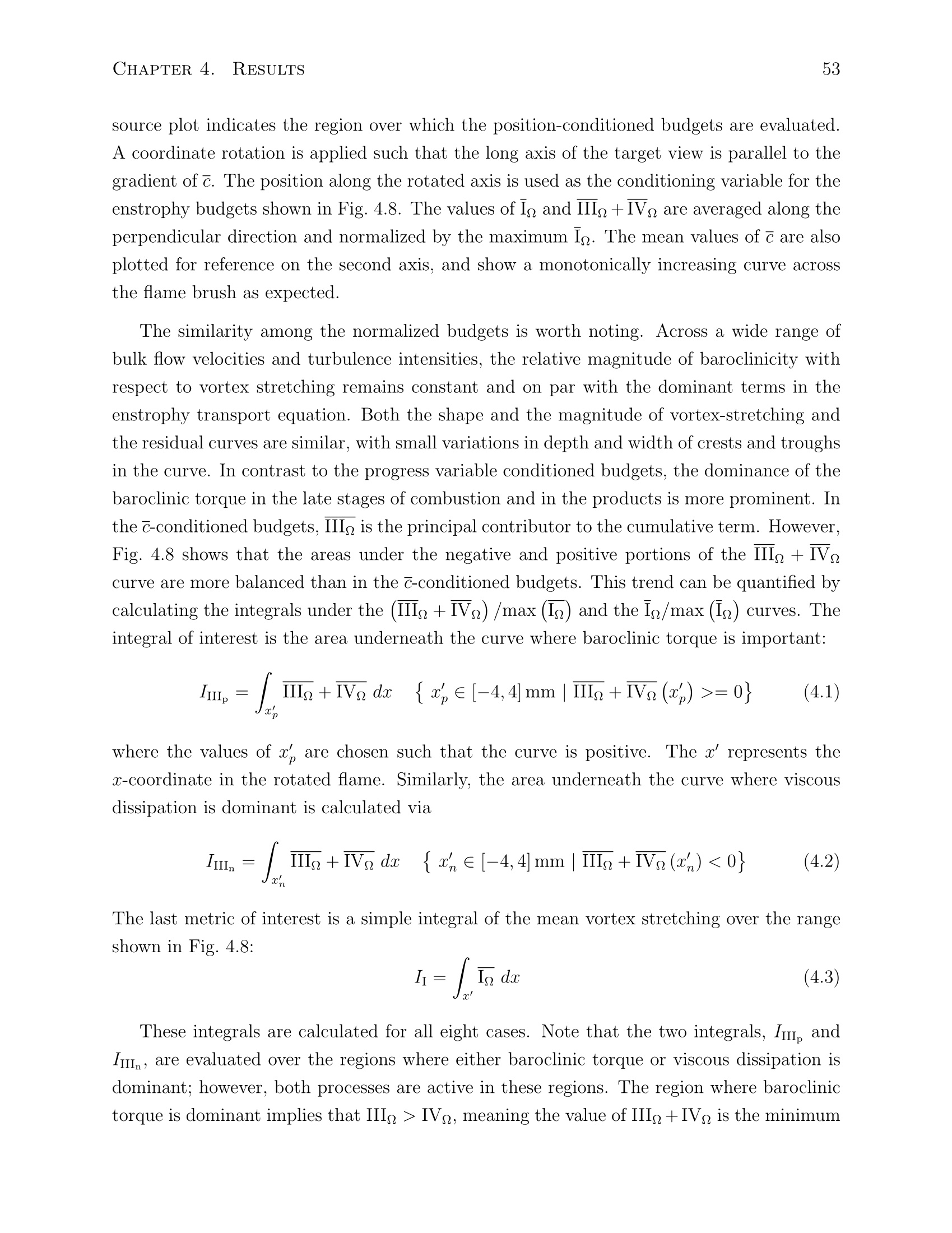
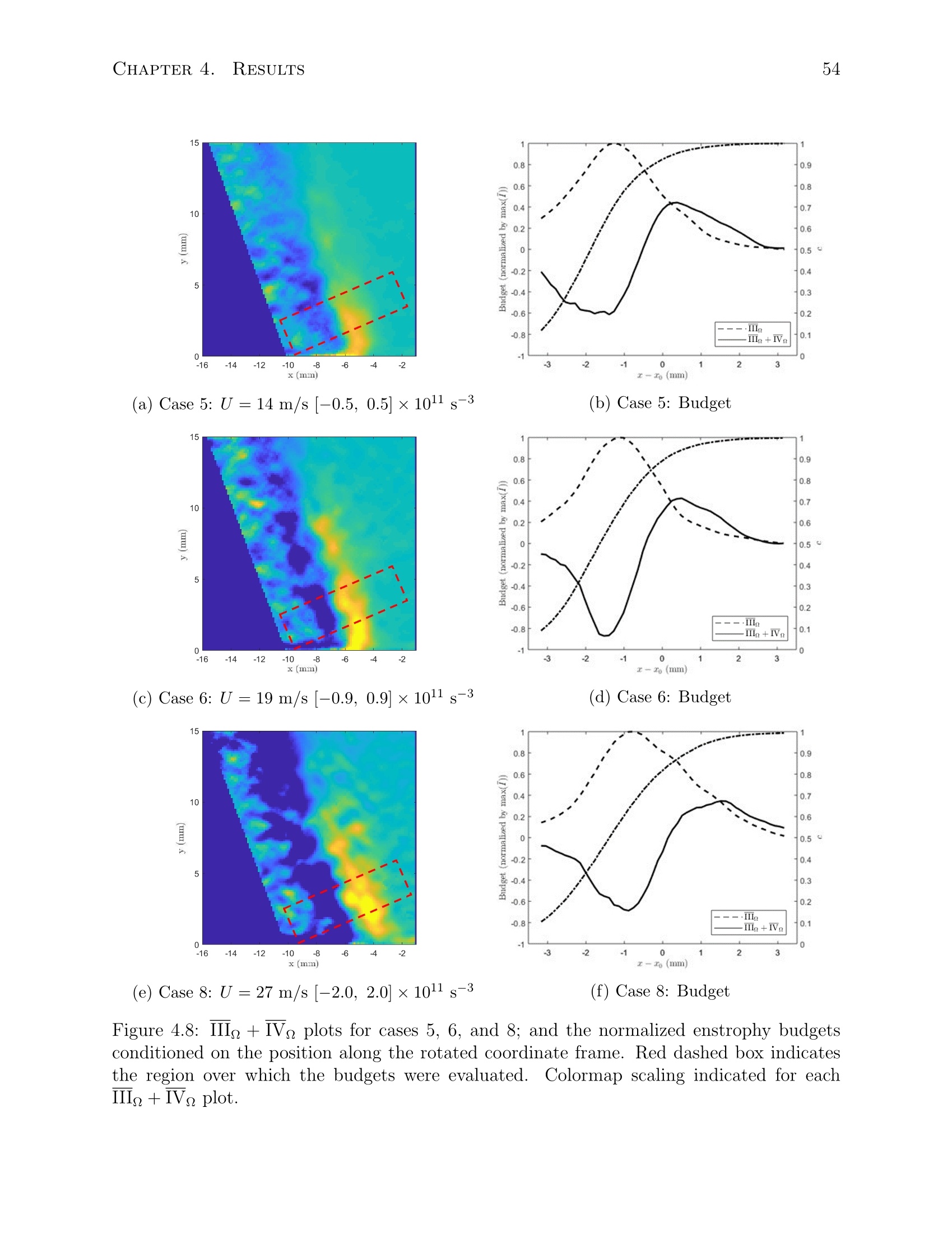
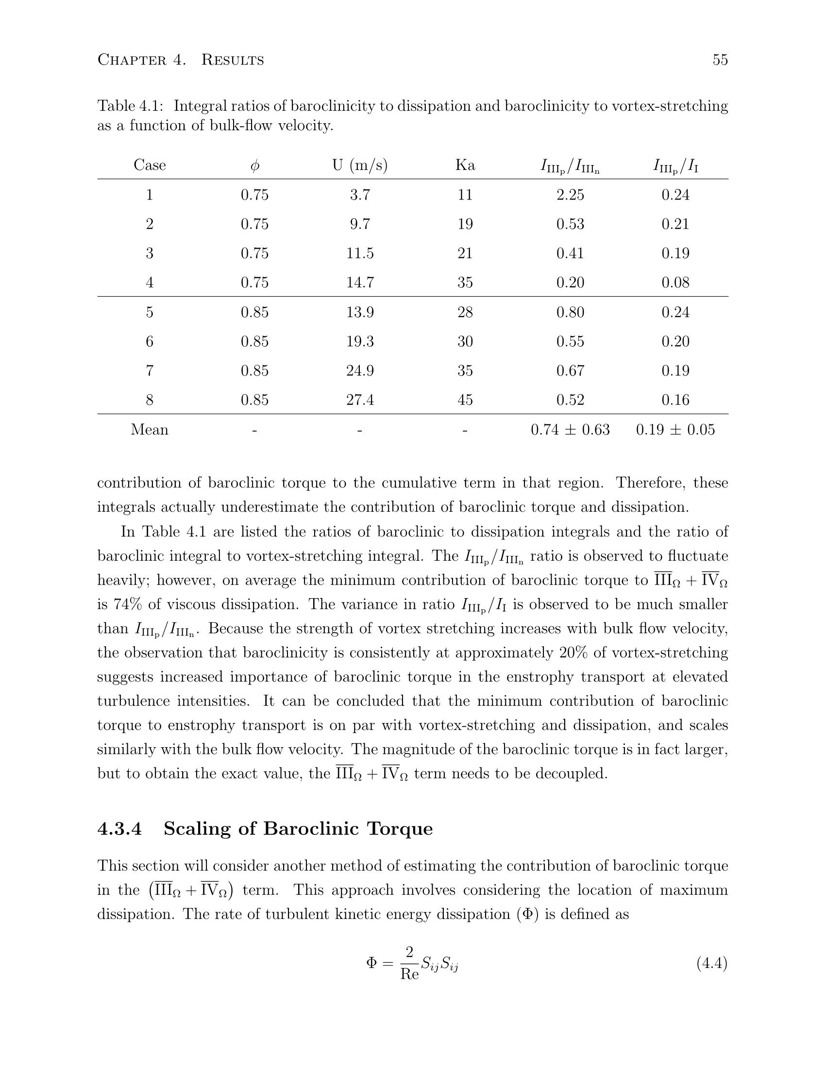
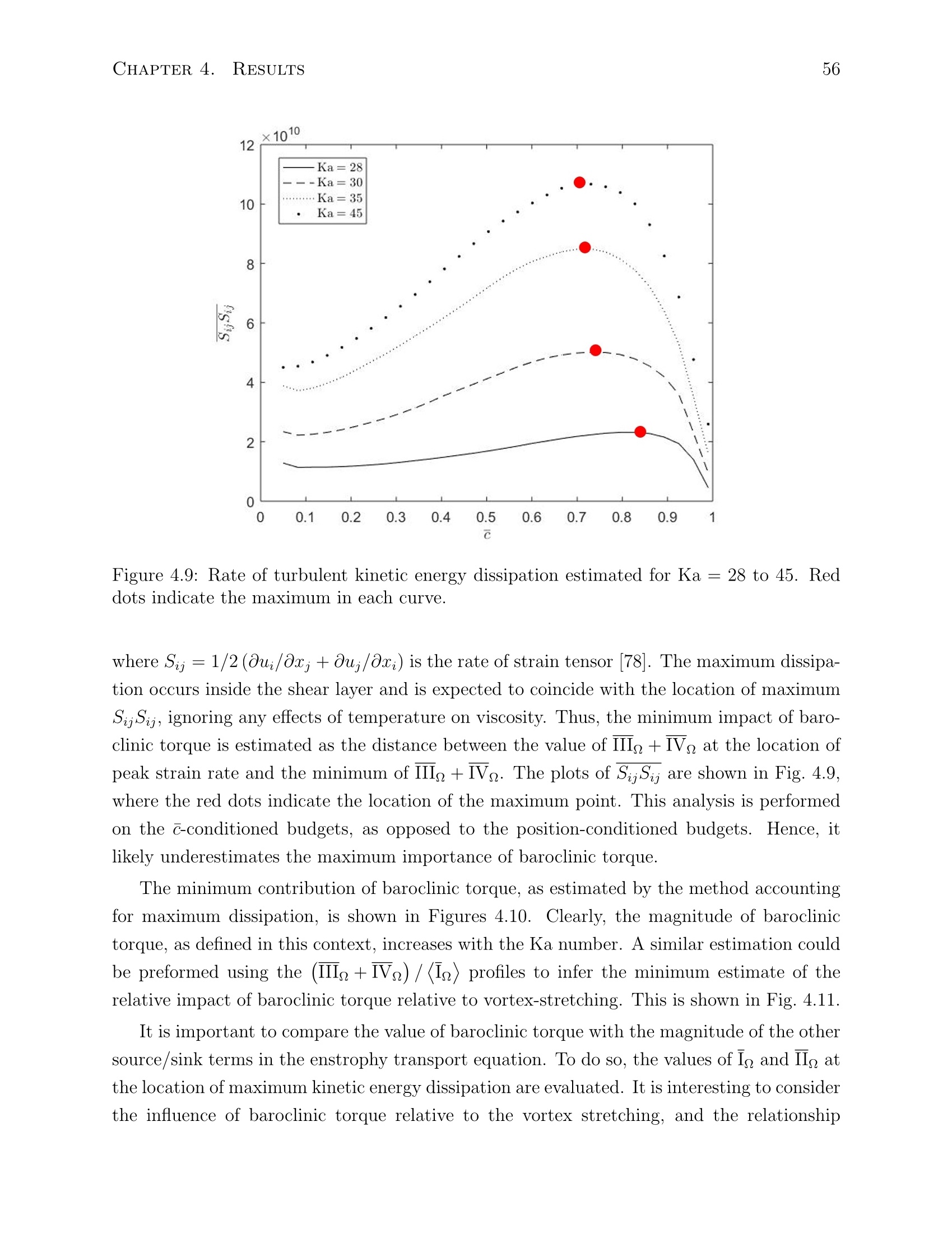
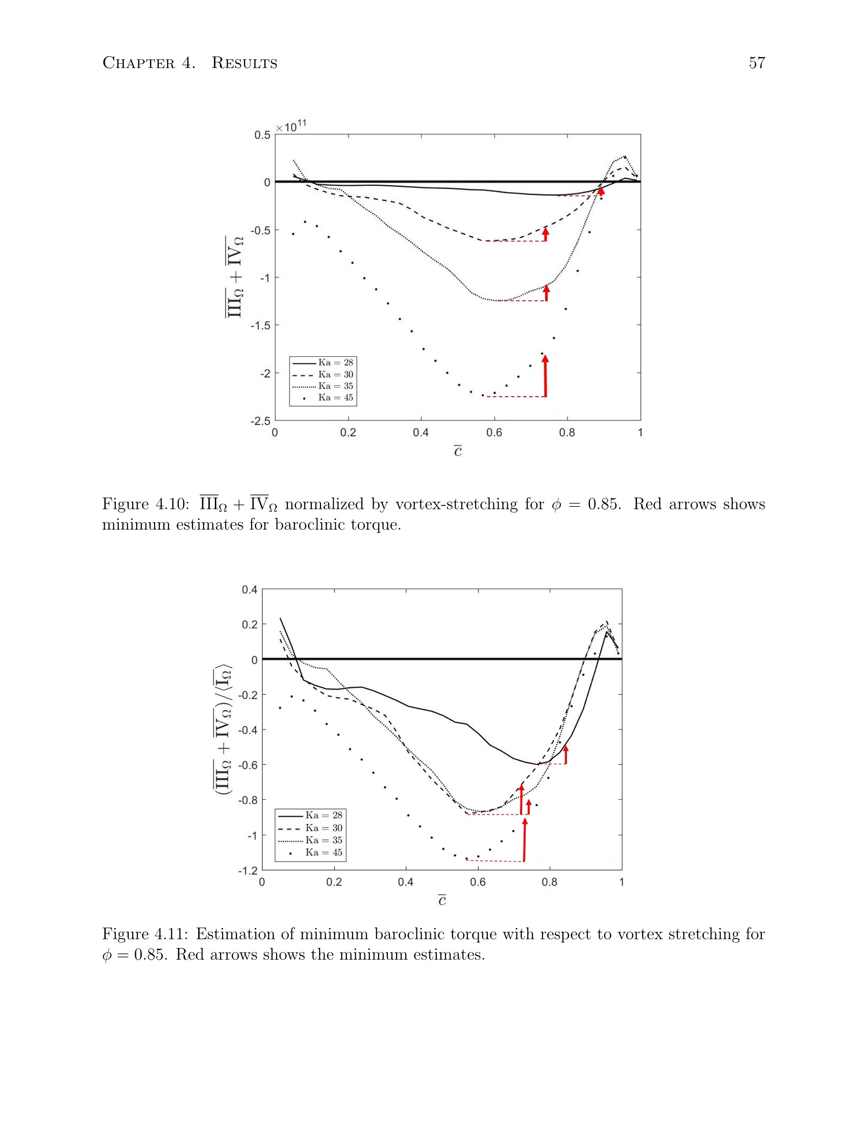
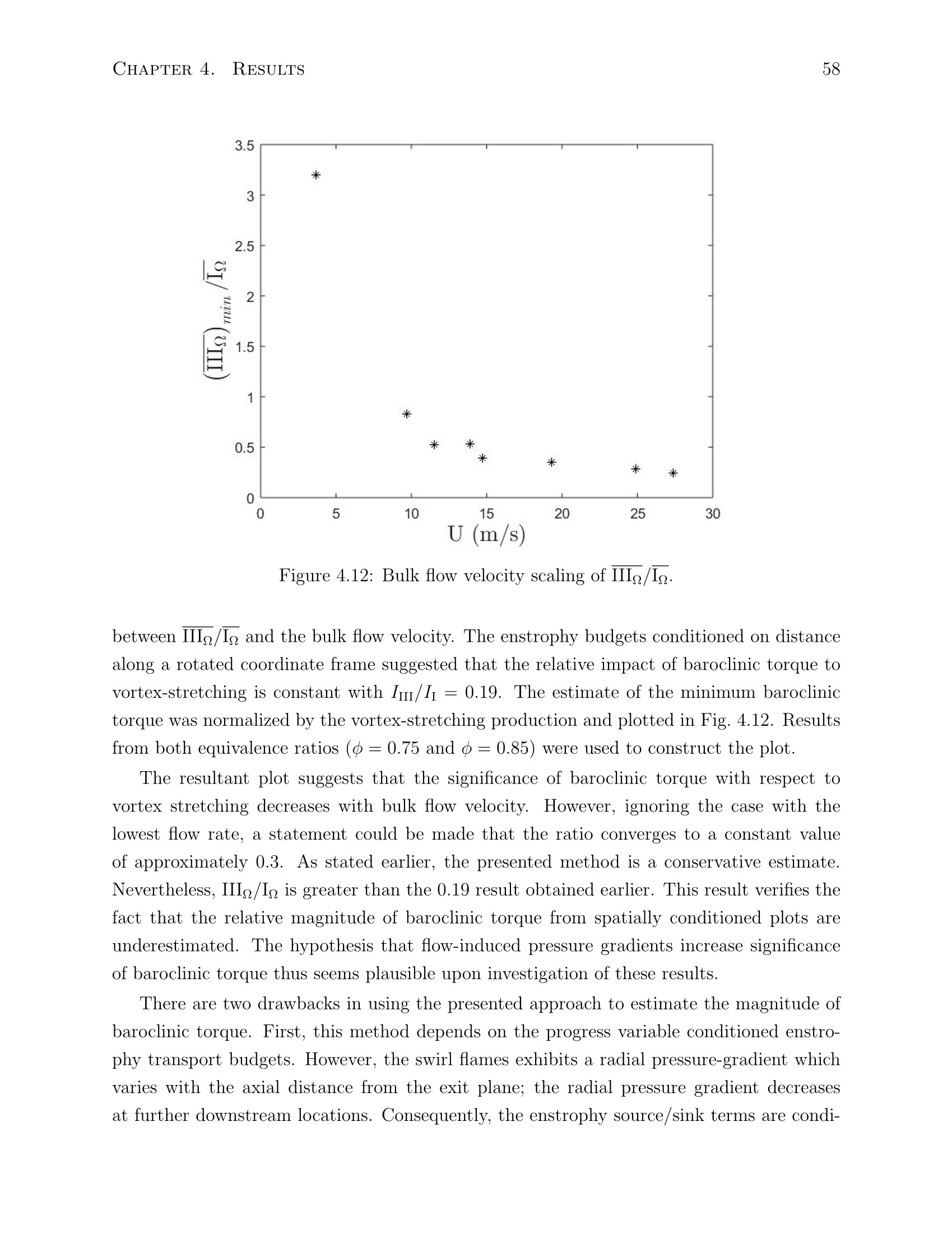
还剩78页未读,是否继续阅读?

产品配置单

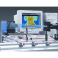
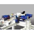

北京欧兰科技发展有限公司为您提供《预混漩涡火焰中显微层析PIV和甲醛的平面激光诱导荧光检测方案(CCD相机)》,该方案主要用于煤炭中显微层析PIV和甲醛的平面激光诱导荧光检测,参考标准--,《预混漩涡火焰中显微层析PIV和甲醛的平面激光诱导荧光检测方案(CCD相机)》用到的仪器有LaVision IRO 图像增强器、PLIF平面激光诱导荧光火焰燃烧检测系统、显微粒子成像测速系统(Micro PIV)、LaVision DaVis 智能成像软件平台
推荐专场
CCD相机/影像CCD
更多




相关方案
更多
该厂商其他方案
更多