水洞中速度矢量场检测方案(粒子图像测速)

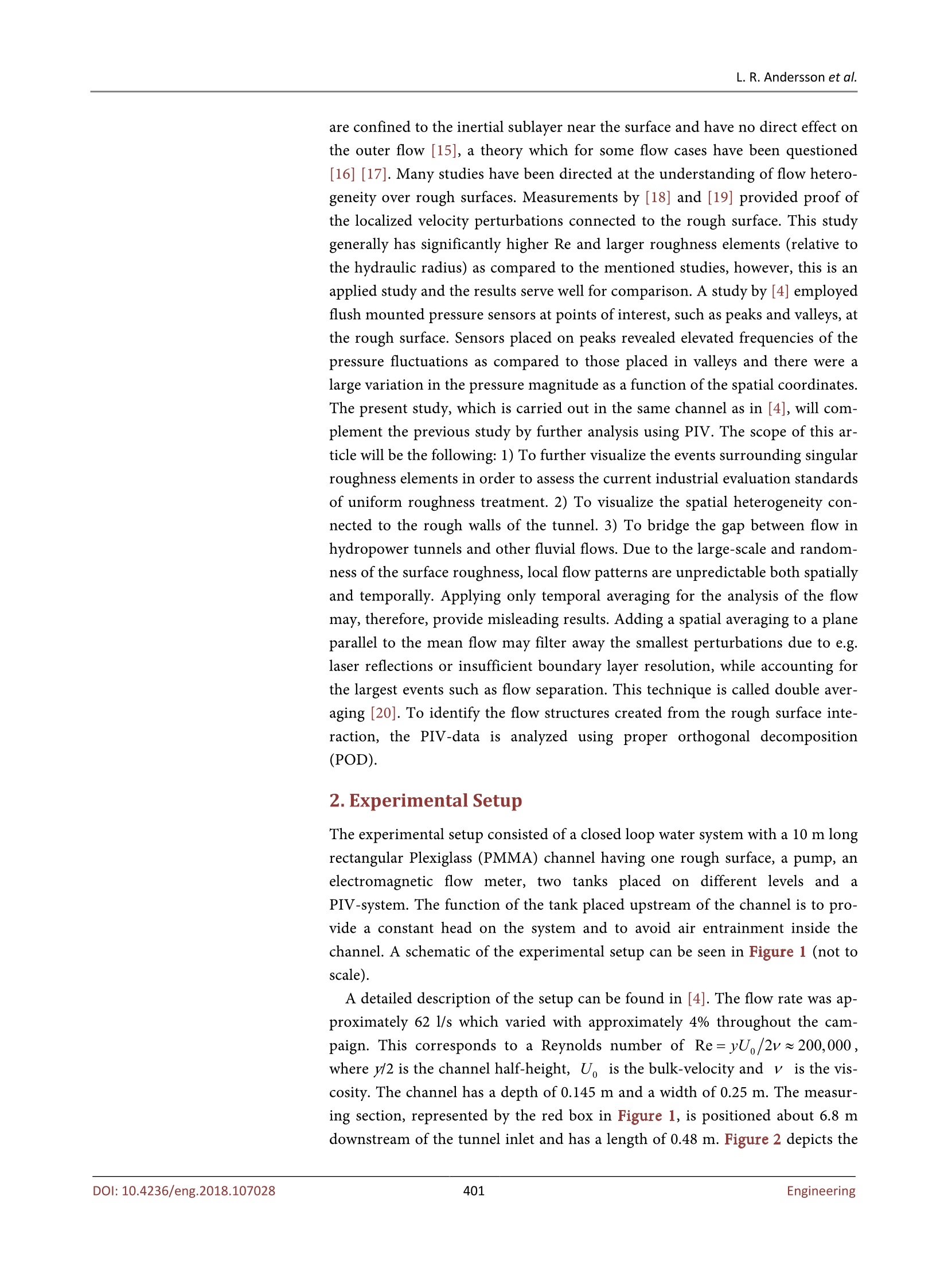
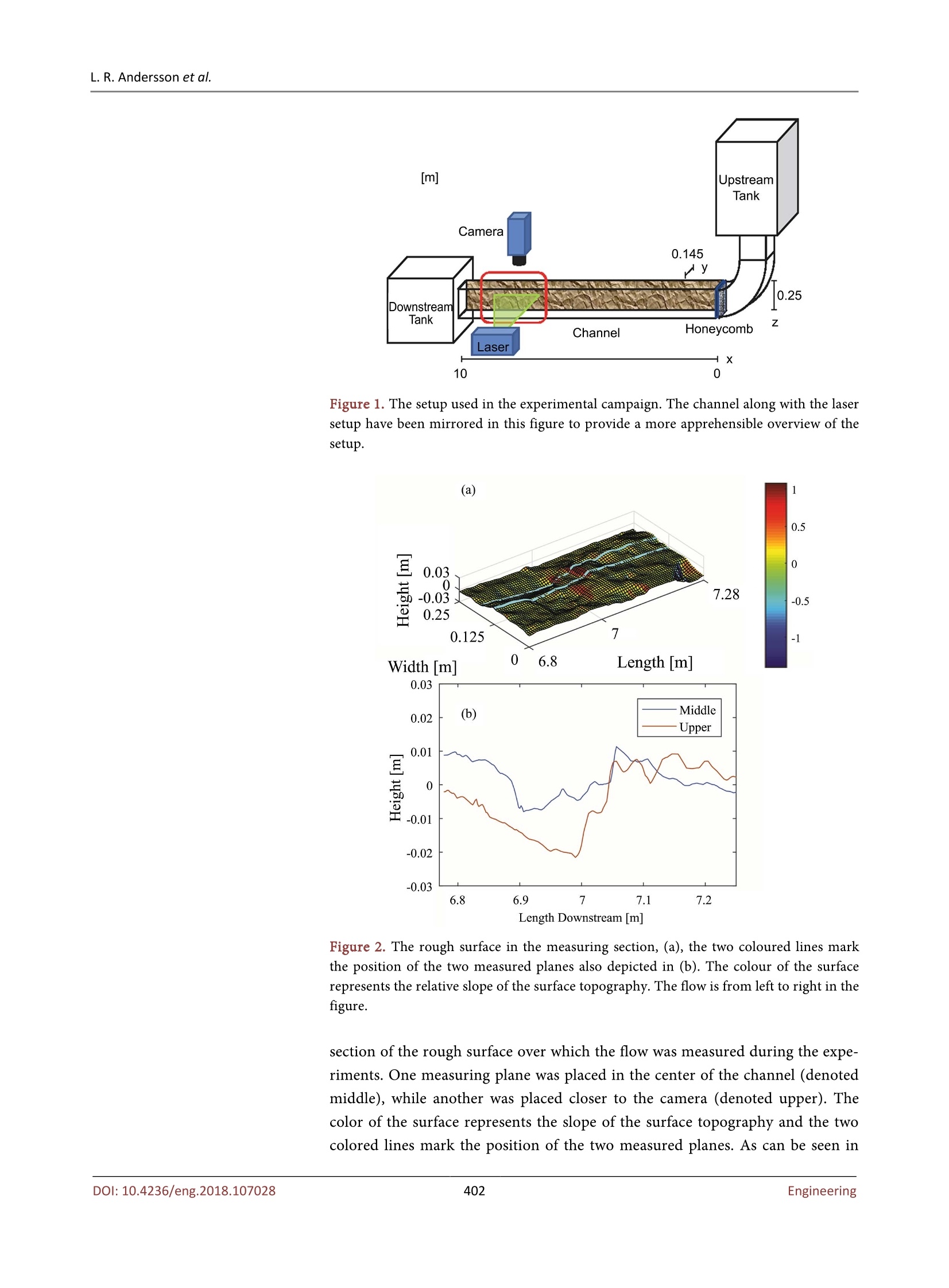
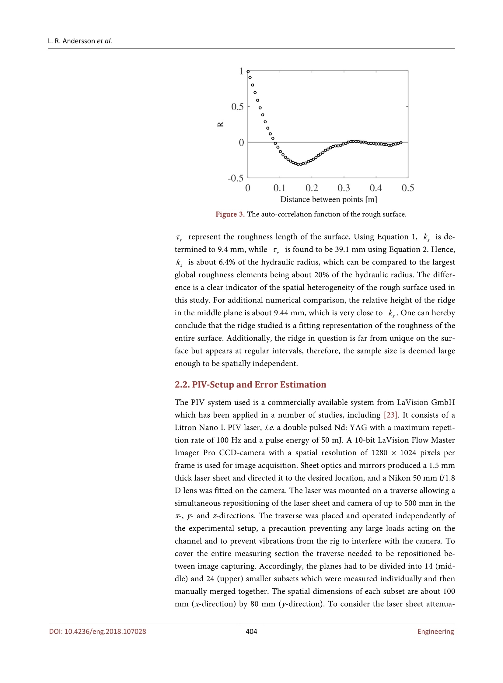
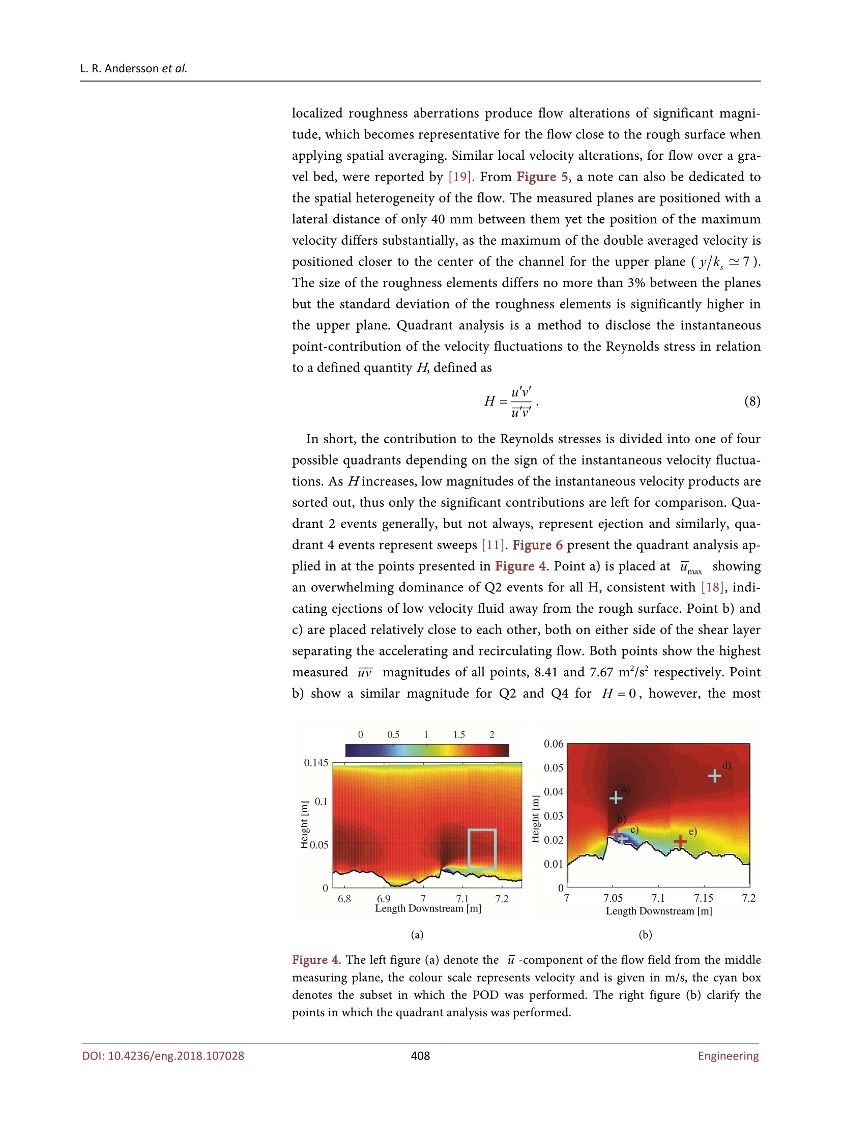
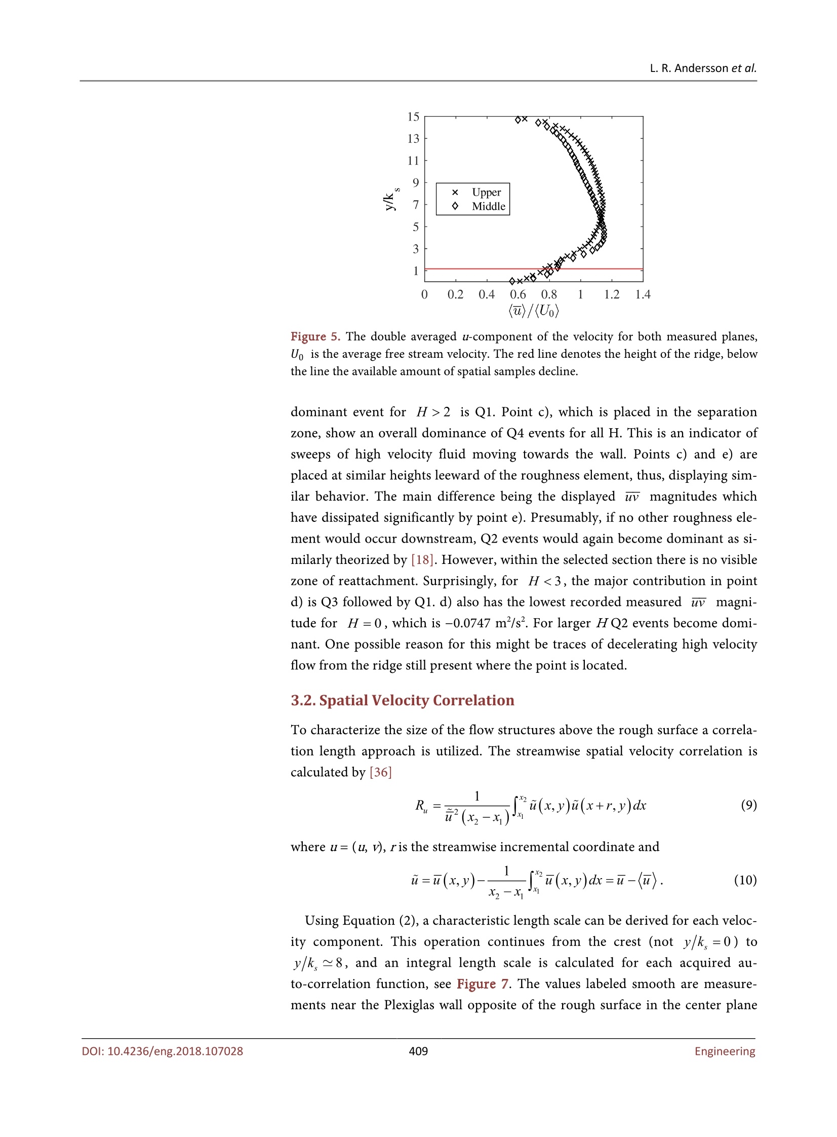
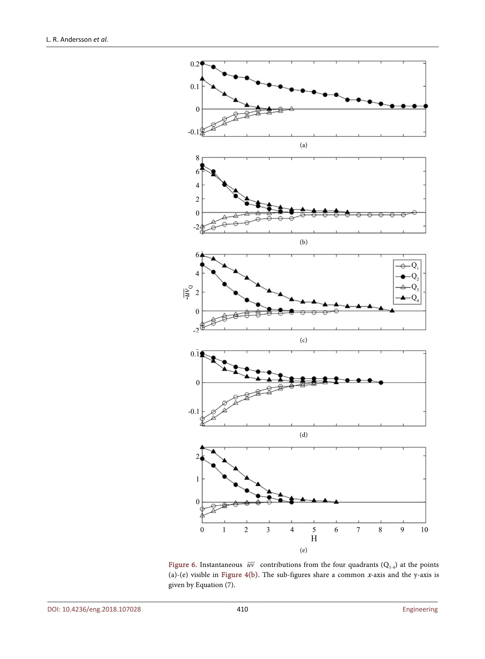
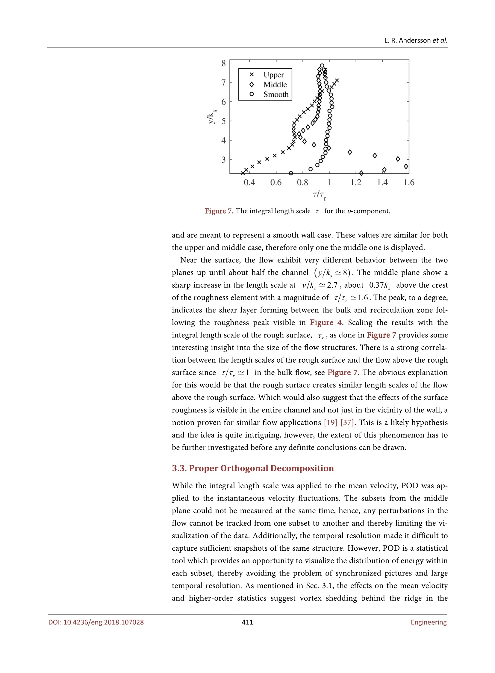
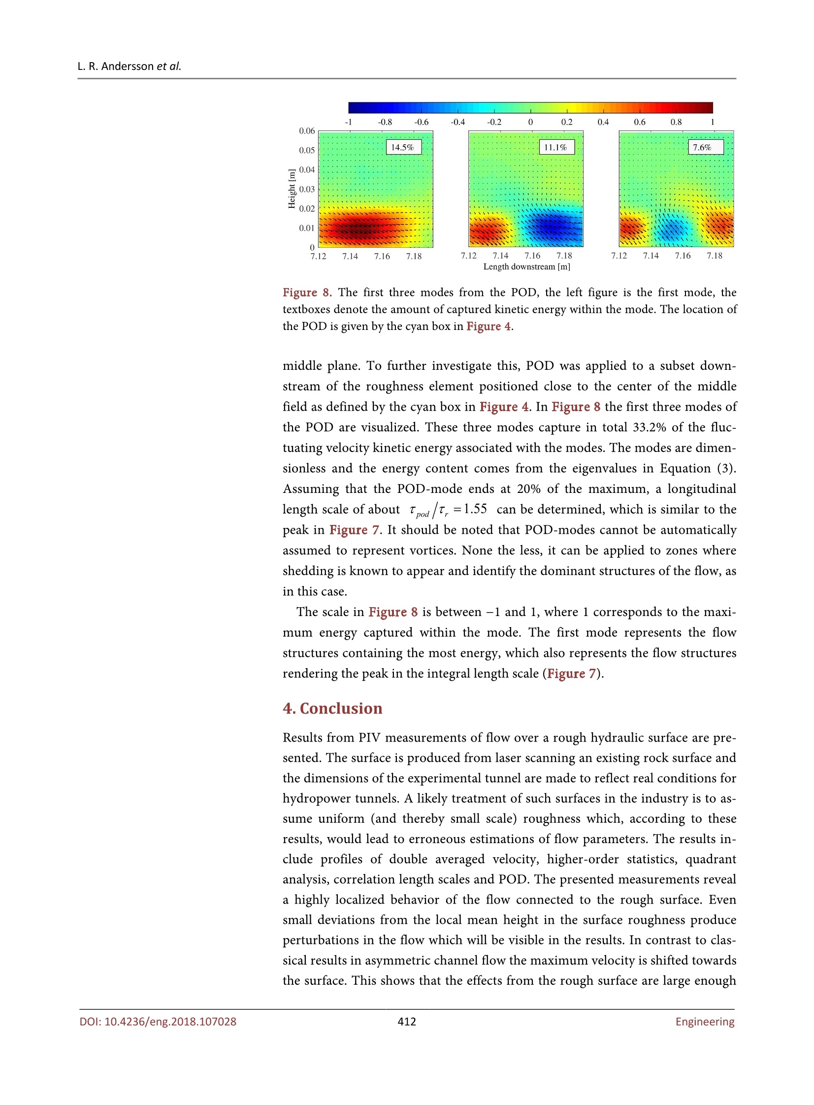
Engineering， 2018， 10， 399-416ScientificResearchPublishinghttp：//www.scirp.org/journal/engISSN Online：1947-394XISSN Print： 1947-3931 L. R. Andersson et al. Characterization of Flow Structures Induced byHighly Rough Surface Using Particle ImageVelocimetry，Proper OrthogonalDecomposition and Velocity Correlations L. R.Andersson1， I. A. S. Larsson1， J. G. I. Hellstrom1， P. Andreasson12， A. G. Andersson1，T.S. Lundstrom1 'Division of Fluid and Experimental Mechanics， Lulea University of Technology， Lulea， SwedenVattenfall Research and Development， Alvkarleby， Sweden Email： robin.andersson@ltu.se How to cite this paper： Andersson， L.R.，Larsson， I.A.S.， Hellstrom， J.G.I.， Andreas-son， P.， Andersson， A.G. and Lundstrom，T.S. (2018) Characterization of FlowStructures Induced by Highly Rough Sur-face Using Particle Image Velocimetry，Proper Orthogonal Decomposition and Ve-locity Correlations. Engineering， 10， 399-416.https：//doi.org/10.4236/eng.2018.107028 Received： June 5，2018 Accepted： July 9， 2018 Published： July 12， 2018 Copyright @ 2018 by authors and Scientific Research Publishing Inc. This work is licensed under the CreativeCommons Attribution International License (CC BY 4.0). http：//creativecommons.org/licenses/by/4.0/Open Access Abstract High Reynolds number flow inside a channel of rectangular cross section isexamined using Particle Image Velocimetry. One wall of the channel has beenreplaced with a surface of a roughness representative to that of real hydro-power tunnels， i.e. a random terrain with roughness dimensions typically inthe range of ~10%-20% of the channels hydraulic radius. The rest of thechannel walls can be considered smooth. The rough surface was capturedfrom an existing blasted rock tunnel using high resolution laser scanning andscaled to 1：10. For quantification of the size of the largest flow structures，integral length scales are derived from the auto-correlation functions of thetemporally averaged velocity. Additionally， Proper Orthogonal Decomposi-tion (POD) and higher-order statistics are applied to the instantaneous snap-shots of the velocity fluctuations. The results show a high spatial heterogeneityof the velocity and other flow characteristics in vicinity of the rough surface，putting outer similarity treatment into jeopardy. Roughness effects are notconfined to the vicinity of the rough surface but can be seen in the outer flowthroughout the channel， indicating a different behavior than postulated byTownsend’s similarity hypothesis. The effects on the flow structures vary de-pending on the shape and size of the roughness elements leading to a highspatial dependence of the flow above the rough surface. Hence， any spatial av-eraging， e.g. assuming a characteristic sand grain roughness factor， for deter-mining local flow parameters becomes less applicable in this case. Keywords CFD， Validation， Hydraulic Roughness，PIV， Hydropower 1.Introduction Water tunnels are frequently used to convey water to and from hydropower tur-bines and in other sectors of infrastructure. The tunnels are often a key part ofthe design and their durability is vital for the continued operation. Tunnel exca-vation by rock-blasting is a relatively swift， and therefore popular， method com-pared to using tunnel boring machines [1]. One significant drawback of the me-thod would be that the resulting walls of the tunnels have varying cross sectionand considerable surface roughness [2]. The scales of roughness in unlined hy-dropower tunnels range from a few millimeters to meters， which may be in therange of ~10%- 20% of the hydraulic radius. A likely treatment of rough wallsby today's industrial standards is to estimate the roughness from the actualphysical features of the roughness， e.g. estimates according to Manning， Chezy，grain size distribution [3]. These approaches have a long track record but onlyprovide spatially averaged quantities and nothing about the actual dynamicswithin the tunnel. The physics of the flow in highly rough tunnels includes largevariations and gradients of pressure[4] and velocity [5]， resulting in intermittentpressure forces and increased local shearing load acting on the walls of the tun-nel. Such forces may very well jeopardize the structural integrity of the walls，causing events including erosion or even partial collapse of the tunnel [6]. Col-lapsing hydropower tunnels is a known problem and documented cases showthat even after 30 - 40 years of usage some tunnels have experienced sudden se-vere failure [7]. The connection between the details of the flow and fatal failureof tunnels is not completely understood， but it has been theorized that intermit-tent pressure fluctuations directly coupled to surface roughness may have in-duced or facilitated the process. Similar results were presented in a recent studyby [8]， showing that pressure-driven cyclic injection of fluid into rock materialleads to larger damage， and at lower pressure than by static injection. Hydro-power tunnels are a very hostile environment to measure within， hence， accurateresults are almost non-existing. Capturing the geometry of existing tunnels alsopresents several problems： The tunnels themselves are dark and humid， makingaccurate measurements difficult [1]. Closing down the tunnels， and thereby anymachinery operating downstream， is very expensive and puts the system in dan-ger [6]. Therefore， there exist very few cases where experiments have been per-formed on models reflecting actual tunnels. This problem was highlighted by [9]but to a degree still remain today. It is well established that rough walls modify the behavior of the flow [10]，[11] however to what extent has been thoroughly debated. For rough surfaces，the turbulence is associated with shear layers formed at the crests of the rough-ness elements where flow separation may occur [12]. For surfaces of sufficientlylarge roughness， individual surface aberrations frequently penetrate into the in-ertial sublayer [13] [14] leading to a breakdown of the logarithmic law of thewall. Yet to this day，a common way to model flow in hydropower tunnels inindustry is to replace the natural roughness with numerical wall-roughnessfunctions. This method relies on the conventional concept that roughness effects are confined to the inertial sublayer near the surface and have no direct effect onthe outer flow [15]， a theory which for some flow cases have been questioned[16] [17]. Many studies have been directed at the understanding of flow hetero-geneity over rough surfaces. Measurements by [18] and [19] provided proof ofthe localized velocity perturbations connected to the rough surface. This studygenerally has significantly higher Re and larger roughness elements (relative tothe hydraulic radius) as compared to the mentioned studies， however， this is anapplied study and the results serve well for comparison. A study by [4] employedflush mounted pressure sensors at points of interest， such as peaks and valleys， atthe rough surface. Sensors placed on peaks revealed elevated frequencies of thepressure fluctuations as compared to those placed in valleys and there were alarge variation in the pressure magnitude as a function of the spatial coordinates.The present study， which is carried out in the same channel as in [4]， will com-plement the previous study by further analysis using PIV. The scope of this ar-ticle will be the following： 1) To further visualize the events surrounding singularroughness elements in order to assess the current industrial evaluation standardsof uniform roughness treatment. 2) To visualize the spatial heterogeneity con-nected to the rough walls of the tunnel. 3) To bridge the gap between flow inhydropower tunnels and other fluvial flows. Due to the large-scale and random-ness of the surface roughness， local flow patterns are unpredictable both spatiallyand temporally. Applying only temporal averaging for the analysis of the flowmay， therefore， provide misleading results. Adding a spatial averaging to a planeparallel to the mean flow may filter away the smallest perturbations due to e.g.laser reflections or insufficient boundary layer resolution， while accounting forthe largest events such as flow separation. This technique is called double aver-aging [20]. To identify the flow structures created from the rough surface inte-raction， the PIV-data is analyzed using proper orthogonal decomposition(POD). 2. Experimental Setup The experimental setup consisted of a closed loop water system with a 10 m longrectangular Plexiglass (PMMA) channel having one rough surface， a pump， anelectromagnetic flow meter， two tanks placed on different levels andaPIV-system. The function of the tank placed upstream of the channel is to pro-vide a constant head on the system and to avoid air entrainment inside thechannel. A schematic of the experimental setup can be seen in Figure 1 (not toscale). A detailed description of the setup can be found in [4]. The flow rate was ap-proximately 62 l/s which varied with approximately 4% throughout the cam-paign. This corresponds to a Reynolds number of Re=yU，/2v~200，000，where y/2 is the channel half-height， U is the bulk-velocity and v is the vis-cosity. The channel has a depth of 0.145 m and a width of 0.25 m. The measur-ing section， represented by the red box in Figure 1， is positioned about 6.8 mdownstream of the tunnel inlet and has a length of 0.48 m. Figure 2 depicts the Figure 1. The setup used in the experimental campaign. The channel along with the lasersetup have been mirrored in this figure to provide a more apprehensible overview of thesetup. (a) 0.5 0 -0.5 Length Downstream [m] Figure 2. The rough surface in the measuring section， (a)， the two coloured lines markthe position of the two measured planes also depicted in (b). The colour of the surfacerepresents the relative slope of the surface topography. The flow is from left to right in thefigure. section of the rough surface over which the flow was measured during the expe-riments. One measuring plane was placed in the center of the channel (denotedmiddle)， while another was placed closer to the camera (denoted upper). Thecolor of the surface represents the slope of the surface topography and the twocolored lines mark the position of the two measured planes. As can be seen in the figure， a ridge is passing through both measuring planes at x~ 7.06 m. Theridge is of interest for the measurements since the maximum height relative to y=0 (the mean height) is similar for the two lines， additionally， the gradient ofthe surface is also nearly the same. However， the relative size of the ridge differssignificantly between the lines. For the blue line defining the middle plane， thefinal slope of the ridge is very sharp but the roughness leading up to the elementis relatively small， consequently， the relative size of the roughness element issmall. On the red line (upper plane)， the ridge is preceded by a“valley”， makingthe relative height larger. Ideally， four rough walls would have been used to keepthe setup as realistic as possible. However， PIV requires optical access from atleast 2 directions and therefore only one rough wall was used. In this study， a right-handed coordinate system is employed with thex-coordinate (u-velocity component) originating from the tunnel entrancepointing in the flow direction. The y-coordinate (v-velocity component) is per-pendicular to the rough surface with y=0 defined as the average elevation of therough surface， hence all presented heights are relative to the average height ofthe surface. Accordingly， the z-coordinate originates from the bottom wall in theflow direction. 2.1. The Rough Surface Model The rough surface model used in the experiments is a 1：10 scale side wall of anexisting rock tunnel whose topography has been captured by high resolution la-ser scanning， a method which has been proven efficient for determining surfaceroughness [1]. One of the main characteristics used to describe a rough surfaceis the height distribution function p(k)， in this case the Gaussian distribution.The meaning of p(k) is that the probability of any surface height between kand k+dkis p(k)dk[21]. Another important factor for characterizing arough surface is the root mean square (RMS) roughness factor， which describesthe average elevation of the roughness elements on the surface. In the currentstudy the RMS roughness factor is denoted as the equivalent sand grain rough-ness factor k for the surface and is defined as [1][22] As mentioned， k. is solely based on the height on the rough surface and doesnot take into consideration e.g. shape or aspect ratio of the roughness. To eva-luate the spatial difference， the auto-correlation function R(r) over a specifiedlength L is introduced in the stream wise direction (x-direction) of the roughsurface [21]. The result can be seen in Figure 3， which is a z-direction average ofthe autocorrelation function. Integrating the auto-correlation function according to Equation (2) producesthe integral length scale of the surface Conclusively， k， is a quantity representative for the roughness height while Figure 3. The auto-correlation function of the rough surface. t， represent the roughness length of the surface. Using Equation 1， k is de-termined to 9.4 mm， while t， is found to be 39.1 mm using Equation 2. Hence，k， is about 6.4% of the hydraulic radius， which can be compared to the largestglobal roughness elements being about 20% of the hydraulic radius. The differ-ence is a clear indicator of the spatial heterogeneity of the rough surface used inthis study. For additional numerical comparison， the relative height of the ridgein the middle plane is about 9.44 mm， which is very close to k. One can herebyconclude that the ridge studied is a fitting representation of the roughness of theentire surface. Additionally， the ridge in question is far from unique on the sur-face but appears at regular intervals， therefore， the sample size is deemed largeenough to be spatially independent. 2.2.PIV-Setup and Error Estimation The PIV-system used is a commercially available system from LaVision GmbHwhich has been applied in a number of studies， including [23]. It consists of aLitron Nano L PIV laser， i.e. a double pulsed Nd： YAG with a maximum repeti-tion rate of 100 Hz and a pulse energy of 50 mJ. A 10-bit LaVision Flow MasterImager Pro CCD-camera with a spatial resolution of 1280 × 1024 pixels perframe is used for image acquisition. Sheet optics and mirrors produced a 1.5 mmthick laser sheet and directed it to the desired location， and a Nikon 50 mm f/1.8D lens was fitted on the camera. The laser was mounted on a traverse allowing asimultaneous repositioning of the laser sheet and camera of up to 500 mm in thex-， y- and z-directions. The traverse was placed and operated independently ofthe experimental setup， a precaution preventing any large loads acting on thechannel and to prevent vibrations from the rig to interfere with the camera. Tocover the entire measuring section the traverse needed to be repositioned be-tween image capturing. Accordingly， the planes had to be divided into 14 (mid-dle) and 24 (upper) smaller subsets which were measured individually and thenmanually merged together. The spatial dimensions of each subset are about 100mm (x-direction) by 80 mm (y-direction). To consider the laser sheet attenua- tion in the image periphery， subsequent positions are set to give a 30 mm over-lap of the images. Stitching together the domain using the measured sets maycreate discontinuities in the domain， due to the different sets not matching per-fectly. However by careful stitching， a good statistical convergence and choosingappropriate overlap the largest discrepancy between two sets which was no morethan 1.3% in the streamwise direction. In the spanwise direction， the discrepancyis less than 1%. The tracer particles used were the previously proven feasible [24]Akzo Nobels Expancel 461 WU 20 hollow thermoplastic spheres with a diameterranging from 2 um to 30 um， and a density of 1.2 g/cm. The measurements wereperformed with a frequency of 75 Hz during 9.49 s， corresponding to a total of712 image pairs for each recorded set. To account for the localized variations invelocity and pixel displacement， the time interval between the laser pulsesranged from 150 us -275 us depending on the measuring position. The resultswere a typical mean displacement over the whole velocity field of 0.3 pixels inthe y-direction and 7 pixels in the x-direction with a characteristic particle imagediameter of 2 pixels. At approximately 490 samples the temporally averaged ve-locity converges towards a stable value. Beyond 560 samples the velocity differno more than 1.5% from the converged value. A PIV experimental setup consistsof several sub systems， and hence there are a number of potential error sources.The overall measurement accuracy in PIV is a combination of a variety of as-pects extending from the recording process all the way to the methods of evalua-tion [25]. A cornerstone in all experimental design is to randomize the measur-ing procedure. By proper randomization， the effects of extraneous factors thatmay be present have less impact on the result [26]. The measurement uncertain-ties consist of those due to systematic biased errors and random precision errors(or due to erroneous measurements) [27]. The biased error associated with thescaling from pixels to meters is estimated to be 0.5% as derived from measure-ments over a known length scale. The primary source of random error is intro-duced by the sub-pixel estimator in the cross-correlation. This error is estimatedto be 10% of the particle image diameter， which is the diameter in pixels of theparticle as seen through the camera [28]. The mean particle image diameter inthe present case is about 2 pixels， and a typical displacement between imagepairs is 7 pixels in the main flow direction. Therefore the estimated random er-ror of the measured velocity vector in each interrogation area is about 4% for thestreamwise velocity component. The rough surface reflected light from the laserwhich in some images saturated the camera， inhibiting measurements of thenear-wall flow. However， these effects where highly localized and within0≤y/k，<1 of the rough surface， and hence， never affected the bulk-flow. Sincethe rough surface was placed on a side wall of the channel， the camera wasplaced above the channel facing downward， see Figure 1. The roughness ele-ments closer to the camera sometimes covered parts of the plane intended formeasuring， generating additional difficulties in measuring the near wall behaviorof the flow. The laser sheet was initially positioned at the center of the channel(middle plane) to get a measurement where the effect of the side walls was as small as possible， and to get a measurement over a distinct roughness element.The second measurement section (upper) was placed at the same x-coordinate asthe first one but closer to the camera， see Figure 2. 2.3. PIVPost-Processing Post-processing of the PIV-data was done using the commercial software DaVisby LaVision [29]. To calculate the particle displacement， a min/max filter forparticle intensity normalization followed by a multi-pass scheme with decreasingwindow size and offset was used. The interrogation window size was 32 × 32pixels for the first pass and 16× 16 pixels for the second pass with adaptivewindow shift， both with an overlap of 25%. The cross-correlation was performedusing the standard cyclic FFT-algorithm with a three-point Gaussian peak fit toestimate the sub-pixel displacement， followed by vector post-processing by ap-plying a median filter to reject spurious vectors (less than 2%) and to interpolatefrom surrounding interrogation windows [30]. The processed data were im-ported into Matlab using PIV mat where further analysis was performed. Thedouble averaging process is performed through two decompositions， the firstpart is the Reynolds decomposition where 0=0+0'.6iiss the temporally av-eraged quantity and 0’is the quantity fluctuating in time. The second part isthe spatial decomposition， 0=(0)+6 where the angle brackets denote spatialaveraging over the desired plane and tilde denotes the temporal deviation fromthe double averaged component (). The Reynolds decomposition is appliedwhen post-processing the raw PIV-images， while the spatial decomposition isapplied a posteriori on the processed PIV images. POD is an algorithm whichdetermines and hierarchically ranks the dominant structures in the flow withrespect to their energy content， allowing the statistical capture of flow structuresdespite eventual shortcomings such as insufficient temporal resolution and/orsample size. The POD modes stem from calculation of the singular eigenvaluedecomposition of the auto covariance matrix K， given by i is the total number of eigenvalues， U is a matrix where the columns consist ofthe instantaneous fluctuating velocity snapshots， according to where u；=u；-u for j={1，2...N}. N，/， is the number of snapshots， 712 inthe current case. The modes are then calculated and normalized by The method stems from [31] and a more recent introduction to POD can befound in [32]. 3. Results and Discussion The middle plane is placed at z = 125 mm， and is represented by a diamondsymbol in the figures. The upper plane was placed at z=165 mm and will berepresented by an x symbol in the figures. To avoid cluttering only a portion ofthe data have been plotted， typically every fourth point. This does not affect theresults and is solely for the purpose of making the data easier to distinguish. Thevelocity components of the flow (u， v) are denoted as the vector u. To evaluatethe flow the u- and v-components of the velocity were averaged over time forone measurement (see Sec. 2.) to produce the temporally averaged velocitycomponents u. Some of the results are then spatially averaged in the stream-wise direction， denoted by (u). In the first section below， temporally averagedand Quadrant analysis of the velocity to discern the spatial heterogeneity of theflow are presented. In the second section， integral length scales applied to thetemporally averaged velocity are discussed and in the third section POD is ap-plied on the instantaneous velocity field. The instantaneous contribution to theReynolds stresses are calculated according to where S is a sorting term. If uv falls into quadrant Qthen S= 1， otherwise S=0. T is the total measuring time for each sample. An introduction to Quadrantanalysis can be found in [33] or [11]. 3.1. Average Velocity and Quadrant Analysis Figure 3 shows the u-component of the time averaged velocity field of the mid-dle measurement plane. The flow field above the rough surface exhibits a highlylocalized behavior induced by roughness elements， exemplified by the zone ofhigh velocity formed at the crest of the roughness element (the ridge) positionedatx≈7.06m. The average bulk velocity in the channel is U= 1.562 m/s. A zone of negativevelocity (recirculation zone) is present behind the crest of the ridge， an effect si-milarly visualized by [18]. Consistent with the previously mentioned study， thenegative horizontal flow in the separation zone is about -0.15U . The asymmetric channel flow case (one rough wall opposite of a smooth one)has been well documented by [34]. Traditionally， the rough surface acts as a sinkfor momentum for the flow， due to the outer similarity treatment the velocityclose to the surface can then be approximated using the logarithmic law of thewall. Accordingly， the maximum of the double averaged streamwise velocitycomponent is shifted away from the rough surface [35]. For the current case， the maximum velocity umax =1.45U is shifted towardsthe rough surface (y/k =4.1) (see Figure 5)， similar to the results of [24]. The localized roughness aberrations produce flow alterations of significant magni-tude， which becomes representative for the flow close to the rough surface whenapplying spatial averaging. Similar local velocity alterations， for flow over a gra-vel bed， were reported by [19]. From Figure 5， a note can also be dedicated tothe spatial heterogeneity of the flow. The measured planes are positioned with alateral distance of only 40 mm between them yet the position of the maximumvelocity differs substantially， as the maximum of the double averaged velocity ispositioned closer to the center of the channel for the upper plane (y/k=7).The size of the roughness elements differs no more than 3% between the planesbut the standard deviation of the roughness elements is significantly higher inthe upper plane. Quadrant analysis is a method to disclose the instantaneouspoint-contribution of the velocity fluctuations to the Reynolds stress in relationto a defined quantity H， defined as In short， the contribution to the Reynolds stresses is divided into one of fourpossible quadrants depending on the sign of the instantaneous velocity fluctua-tions. As Hincreases， low magnitudes of the instantaneous velocity products aresorted out， thus only the significant contributions are left for comparison. Qua-drant 2 events generally， but not always， represent ejection and similarly， qua-drant 4 events represent sweeps [11]. Figure 6 present the quadrant analysis ap-plied in at the points presented in Figure 4. Point a) is placed atumax showingan overwhelming dominance of Q2 events for all H， consistent with [18]， indi-cating ejections of low velocity fluid away from the rough surface. Point b) andc) are placed relatively close to each other， both on either side of the shear layerseparating the accelerating and recirculating flow. Both points show the highestmeasureduv magnitudes of all points， 8.41 and 7.67 m/s’ respectively. Pointb) show a similar magnitude for Q2 and Q4 for H=0， however， the most (a) (b) Figure 4. The left figure (a) denote the u -component of the flow field from the middlemeasuring plane， the colour scale represents velocity and is given in m/s， the cyan boxdenotes the subset in which the POD was performed. The right figure (b) clarify thepoints in which the quadrant analysis was performed. Figure 5. The double averaged u-component of the velocity for both measured planes，Uo is the average free stream velocity. The red line denotes the height of the ridge， belowthe line the available amount of spatial samples decline. dominant event for H>2 is Q1. Point c)， which is placed in the separationzone， show an overall dominance of Q4 events for all H. This is an indicator ofsweeps of high velocity fluid moving towards the wall. Points c) and e) areplaced at similar heights leeward ofthe roughness element， thus， displaying sim-ilar behavior. The main difference being the displayed uv magnitudes whichhave dissipated significantly by point e). Presumably， if no other roughness ele-ment would occur downstream， Q2 events would again become dominant as si-milarly theorized by [18]. However， within the selected section there is no visiblezone of reattachment. Surprisingly， for H<3， the major contribution in pointd) is Q3 followed by Q1. d) also has the lowest recorded measured uv magni-tude for H=0， which is -0.0747 m’/s’. For larger H Q2 events become domi-nant. One possible reason for this might be traces of decelerating high velocityflow from the ridge still present where the point is located. 3.2.Spatial Velocity Correlation To characterize the size of the flow structures above the rough surface a correla-tion length approach is utilized. The streamwise spatial velocity correlation iscalculated by [36] where u=(u，v)， ris the streamwise incremental coordinate and Using Equation (2)， a characteristic length scale can be derived for each veloc-ity component. This operation continues from the crest (not y/k=0) toy/k，=8， and an integral length scale is calculated for each acquired au-to-correlation function， see Figure 7. The values labeled smooth are measure-ments near the Plexiglas wall opposite of the rough surface in the center plane 0.2 0.1 0 2A -0.1 (a) 8 6 (d) 2 1 0 0 2 4 56 7 8 10 (e) Figure 6. Instantaneous uv contributions from the four quadrants (Q4) at the points(a)-(e) visible in Figure 4(b). The sub-figures share a common x-axis and the y-axis isgiven by Equation (7). DOI： 10.4236/eng.2018.107028 410 Figure 7. The integral length scale t for the u-component. and are meant to represent a smooth wall case. These values are similar for boththe upper and middle case， therefore only one the middle one is displayed. Near the surface， the flow exhibit very different behavior between the twoplanes up until about half the channel (y/k8). The middle plane show asharp increase in the length scale at y/k，2.7， about 0.37k， above the crestof the roughness element with a magnitude oft/t， ~1.6. The peak， to a degree，indicates the shear layer forming between the bulk and recirculation zone fol-lowing the roughness peak visible in Figure 4. Scaling the results with theintegral length scale of the rough surface，t，， as done in Figure 7 provides someinteresting insight into the size of the flow structures. There is a strong correla-tion between the length scales of the rough surface and the flow above the roughsurface since t/t， =1 in the bulk flow， see Figure 7. The obvious explanationfor this would be that the rough surface creates similar length scales of the flowabove the rough surface. Which would also suggest that the effects of the surfaceroughness is visible in the entire channel and not just in the vicinity of the wall， anotion proven for similar flow applications [19] [37]. This is a likely hypothesisand the idea is quite intriguing， however， the extent of this phenomenon has tobe further investigated before any definite conclusions can be drawn. 3.3. Proper Orthogonal Decomposition While the integral length scale was applied to the mean velocity， POD was ap-plied to the instantaneous velocity fluctuations. The subsets from the middleplane could not be measured at the same time， hence， any perturbations in theflow cannot be tracked from one subset to another and thereby limiting the vi-sualization of the data. Additionally， the temporal resolution made it difficult tocapture sufficient snapshots of the same structure. However， POD is a statisticaltool which provides an opportunity to visualize the distribution of energy withineach subset， thereby avoiding the problem of synchronized pictures and largetemporal resolution. As mentioned in Sec. 3.1， the effects on the mean velocityand higher-order statistics suggest vortex shedding behind the ridge in the Figure 8. The first three modes from the POD， the left figure is the first mode， thetextboxes denote the amount of captured kinetic energy within the mode. The location ofthe POD is given by the cyan box in Figure 4. middle plane. To further investigate this， POD was applied to a subset down-stream of the roughness element positioned close to the center of the middlefield as defined by the cyan box in Figure 4. In Figure 8 the first three modes ofthe POD are visualized. These three modes capture in total 33.2% of the fluc-tuating velocity kinetic energy associated with the modes. The modes are dimen-sionless and the energy content comes from the eigenvalues in Equation (3).Assuming that the POD-mode ends at 20% of the maximum， a longitudinallength scale of about Tpod /t，=1.55 can be determined， which is similar to thepeak in Figure 7. It should be noted that POD-modes cannot be automaticallyassumed to represent vortices. None the less， it can be applied to zones whereshedding is known to appear and identify the dominant structures of the flow， asin this case. The scale in Figure 8 is between -1 and 1， where 1 corresponds to the maxi-mum energy captured within the mode. The first mode represents the flowstructures containing the most energy， which also represents the flow structuresrendering the peak in the integral length scale (Figure 7). 4. Conclusion Results from PIV measurements of flow over a rough hydraulic surface are pre-sented. The surface is produced from laser scanning an existing rock surface andthe dimensions of the experimental tunnel are made to reflect real conditions forhydropower tunnels. A likely treatment of such surfaces in the industry is to as-sume uniform (and thereby small scale) roughness which， according to theseresults， would lead to erroneous estimations of flow parameters. The results in-clude profiles of double averaged velocity， higher-order statistics， quadrantanalysis， correlation length scales and POD. The presented measurements reveala highly localized behavior of the flow connected to the rough surface. Evensmall deviations from the local mean height in the surface roughness produceperturbations in the flow which will be visible in the results. In contrast to clas-sical results in asymmetric channel flow the maximum velocity is shifted towardsthe surface. This shows that the effects from the rough surface are large enough to manifest even in the double averaged velocity. It should be noted that theroughness element studied is not unique， but similar ones occur regularly on therough surface. Therefore， using large spatial samples would produce the samedistortions when averaging. The higher order statistics indicate that the flowabove and behind the ridge is characterized by ejection and intermittent burstsof velocity， this is also where the highest point-contributions to the Reynoldsstresses where recorded. Similarly， earlier measurements showed higher fre-quencies of fluctuating pressure at the same ridge. Research has shown that theseare unfavorable conditions for rock surfaces from a durability point of view andmay hasten or induce an eventual process of tunnel breakdown. As theorized，the problem of tunnel breakdown is likely connected to the flow-roughness ef-fects. Evaluation of the correlation lengths of the flow reveals a significant dif-ference between how the roughness elements interact with the flow. Both theintegral length scales and POD approximately predicted the position of the larg-est flow structures formed in vicinity of the rough surface at y/k，~3. Conse-quently， similar data can be obtained from both the time-averaged velocity andthe instantaneous velocity fluctuations. The streamwise length scales of the flowholds close resemblance to the length scales of the rough surface， since t/t， ≈1for y/k，>7. In contrast to Townsends’s similarity hypothesis where the effectsof the rough surface is visible beyond the range of the rough surface， andthroughout the channel. Similar effects have been shown in studies concerningflow over riverbeds， dunes or in rivers. It should be noted that such cases usuallyemploy lower Re and larger roughness height to surface ratio and would notregularly be associated with the current application. It does， however， highlightthat for hydropower applications， rough surfaces cannot be treated as uniformand only friction-inducing. This is particularly important when modelling flowusing CFD， whose role has grown vastly in many industrial applications the pasttwo decades. The results provided here show that the resolution of the roughnessis very important， which could have large implications on the future evaluationof hydropower tunnels. A different proposed approach would involve a modifi-cation of the uniform wall functions currently used by today's standards. A tho-rough mapping of the turbulent kinetic energy in correlation with the roughsurface would yield the necessary data， as shown by the quadrant analysis in thisstudy. Thereby the law of the wall could be modified with a spatially stochasticlocalized increase in wall-near velocity gradients. The roughness length-scalesemployed in this study might suffice for such an endeavoring as implied by theintegral length-scales， however， different methods of deriving these should nev-ertheless be explored. One limitation of this study is the usage of only one roughwall. Hence， the flow in an actual hydropower tunnel cannot be claimed to befully understood yet， albeit further understood. There has been no indication ofeventual scaling effects between the experiments and the actual case. But if onewould consider the problems within hydropower tunnels today and the agree-ment with other studies the authors assume that the scaling effects， if any， wouldbe insignificant. Acknowledgements The research presented was carried out as a part of “Swedish Hydropower Cen-tre-SVC”. SVC has been established by the Swedish Energy Agency， Energiforskand Svenska Kraftnat together with Lulea University of Technology， KTH RoyalInstitute of Technology， Chalmers University of Technology and Uppsala Uni-versity. ( References ) ( [1] B ratveit， K.， Lia， L. and Olsen，N.R.B. (2012) A n Ef f icient Method to Describe theGeometry a nd the Roughness of an Existing Unlined Hydro Power T u nnelin. Energy Procedia， 20， 200-206. h t tps：//doi.org/10. 1 016/j.egypro.2012.03.02 0 ) ( [2] Perfect， E. (1997) Fractal Models for t he F ragmentation of Rocks and Soils： A Re- view. Engineering Geology，48， 1 85-198. h t tps：// d oi.org/10 .1 016/S0013- 7 952(97)00040-9 ) ( [3] Chanson， H. (2004) T he Hydraulics of Open Channel F l ow： An Introduction， 2nd Edition， Elsevier， Amsterdam. ) ( [4] Andersson， L.R.， L arsson， I .A.S.， Hellstrom， J.G.I.， Andreasson， P. and Andersson，A.G. (2016) Experimental Study of Head Loss over Laser Scanned Rock Tunnelin.6th International Symposium on Hydraulic Str u ctures， Po r tland， 27-30 June 201 6 ， 22-29. ) ( [5] Andersson， L .R.， Hellstrom， J.G.I.， Andreasson ， P . and Andersson， A.G. (2015) Numerical S i mulation of Artificial a nd Natural Rough Surfacesin. AP S 2015 Pro- ceedings，Orlando，20-25 June 2015. ) ( [6] Bratveit， K. ， Bruland， A . and Brevik ， O.(2016) Rock F alls in Selected Norwegian Hydropower Tunnels S u bjected to H ydropeaking. Tunnelling and Underground Space Technology，52，202-207.htt p s：//doi.org/10 . 1016/ j .tust.2015.10.003 ) ( [7] Reinius， E. (1986) Rock Erosion. International Water Power & Dam Construction， 38， 43-48. ) ( [8] Patel， S.M.， Sondergeld， C.H. and Rai， C.S. ( 2 017) Laboratory Studies of H ydraulic Fracturing by Cyclic Injection. International Journal of Rock Mechanics and Min-ing Sciences， 95， 8-15. https：//doi . org/10.1016/j.ijrmms. 2 017 . 03.008 ) ( [9] Grass， A.J. ( 1971) Structural Features of Turbulent Flow over Smooth and R o ugh Boundaries. Journal of Fluid Mechanics，50， 233-255. h tt ps：//doi.o rg /10 . 10 1 7/S0022112071002556 ) ( [10] Jimenez，J.(2004) Turbulent Flows over Rough W alls. Annual Review of Fluid Me-chanics， 36， 173-196. https：//doi.org/10.1 1 4 6/an nu rev.f l uid.36.050802.1 2 2103 ) ( [11] P ope，S.B. ( 2 001) Turbulent Flows. IOP Publishing， Bristol. ) ( [12] K ruse， N.， Kuhn， S. and Rudolf von Rohr， P. ( 2006) Wavy Wall Effects on T u rbu- lence P roduction and Large-Scale Modes. Journal of Turbulence，7， No. 31. ) ( [13] C heng， H. a n d Castro， I.P. (2002) Near Wall Fl o w over Urb a n-Like Roug h ness. Boundary-Layer Meteorology，104，229-259. ht t ps： / /doi.org/ 1 0.1023/A：1016060103 4 4 8 ) ( [14] S chlichting， H. and Gersten， K. (2003) Boundary-Layer Theory. 8th E d ition， Sprin- ger Science， Berlin. ) ( [15] S eddighi， M.， He， S.， Pokrajac， D.， O’donoghue， T . and Vardy，A.E. (2015) Turbu-lence in a Transient Channel F low with a Wall of Pyramid Roughness Journal of Fluid Mechanics， 781，226-260. ) ( [16] K rogstad， P . and Antonia， R. (1999) Surface Roughness E ffects in Turbulent Boun- dary Layers. E xperiments in F l uids， 27， 450-460. https：//doi.org/10 . 1007/s00348005037 0 ) ( [17] P atel， V. (1998) Perspective： Flow at High Reynolds Number and over Rough Sur- f aces-Achilles Heel of CFD. J o urnal of Fluids Engineering， 1 20， 434-444. https：// d oi.org/10.1 11 5 / 1.2820682 ) ( [18] B I ennett， S.J . and Best， J.L. (1995) Mean Flow and Turbulence Structure over Fixed，Two-Dimensional Dunes： Implications for Sediment Transport and Bedform St a - bility. Sedimentology， 42， 491-513. https：//doi.org/10. 111 1/j.1365 - 3091.1995.tb00386.x ) ( [19] B I uffin-Belanger， T.，Ri c e， S. ， Reid， I. and Lancaster，J. (2006) Spatial Heterogeneityof Near-Bed H ydraulics above a Patch o f River Gravel. Water Resources Research， 42， W04413. h ttps：//doi.o r g / 10.1029/2005WR004070 ) ( [20] N ikora， V.， McEwan， I.， Mc L ean， S.， Coleman， S.， P okr a jac， D. and W alte r s， R. (2007) Double-Averaging Concept for Rough-Bed Open-Channel a nd O verland Flows： Theoretical Background. Journal of Hydraulic Engineering， 133，873-883. ht tps：//doi.org/ 1 0 .1061/(AS C E)0733 - 9429(2007 ) 133：8(873) ) ( [21] Z 2 hao， Y .， Wang， G .-C. and Lu， T.-M. ( 2006) Characterization of Amorphous a ndCrystalline Rough S urface： Principles and Applications . Academic P ress， Cam- bridge. ) ( [22] S arkar，S. and Dey， S. (2010) Double-Averaging Turbulence Characteristics in Flows o ver a Gravel Bed. Journal of Hydraulic Research， 48， 801-809. ht t ps：//doi.o rg /10 . 1080/00221686.2010.526764 ) ( [23]I L arsson， I .A.S.， Granstrom， B.R.， Lundstrom， T.S. and Marjavaara， D. (2012) PIV Analysis of Merging Flow in a Rotary Kiln. Experiments in Fluids， 53， 545-560. ) ( [24]/ Andersson， A.G.， A ndreasson， P .， Hellstrom J .G.I. and Lundstrom， T .S. (2012)Modelling and V a lidation of Flow over a Wall with Large Surface Roughness. ) ( [25] R I affel， M.， Willert， C.E. ， Wereley， S.T. and Kompenhans，J. (2007) Particle Image Velocimetry： A P r actical Guide. ) ( [26] M ontgomery， D.C. (2012) D e sign a n d Analysis of E xperiments. ) ( [27 ] C oleman， H.W. an d Steele， W.G. (2009) Experimentation， Va l idation， and Uncer- tainty Analysis for Engineers. 3rd Edition. ) ( 28Balakumar， B .J.， et al. (2009 ) High Resolution Experimental Measurements o fRichtmyer-Meshkov Turbulence in Fluid Layers after Reshock Using Simultaneous PIV-PLIF. P roceedings of the APS Topical Group on Shock Co m pression of Con - densedMatter， Nashville， December 2009， Volume 11 9 5. ht tps：//doi.o rg / 1 0.1063 / 1.3295225 ) ( [29] (2007)LaVision Gmbh Product Manual for Davis 7.2. ) ( [30] W esterweel， J . a nd S c arano， F . ( 2 005) U n iversal Outlier De t ection for PIV Dat a .Experiments in Fluids， 39， 1096-1100. ) ( [31] B I akewell， H.P. (1967) Viscous Sublayer and Adjacent Wall R egion in TurbulentPipe Flow. The Physics of Fluids， 10，1 8 80. ) ( [32] E rik Meyer， K .， Cavar， D. and Pedersen， J.M. ( 2007) POD as T o ol f o r Comparisonof PIV and LES Data. ) [37] Roy， A.G.， Buffin-Belanger， T.， Lamarre， H. and Kirkbride， A.D. (2004) Size， Shapeand Dynamics of Large-Scale Turbulent Flow Structures in a Gravel-Bed River.Journal of Fluid Mechanics， 500， 1-27. https：//doi.org/10.1017/S0022112003006396 OI： eng. Jul. ngineering DOI： eng.ngineering       High Reynolds number flow inside a channel of rectangular cross section is examined using Particle Image Velocimetry. One wall of the channel has been replaced with a surface of a roughness representative to that of real hydropower tunnels, i.e. a random terrain with roughness dimensions typically in the range of ≈10% - 20% of the channels hydraulic radius. The rest of the channel walls can be considered smooth. The rough surface was capturedfrom an existing blasted rock tunnel using high resolution laser scanning and scaled to 1:10. For quantification of the size of the largest flow structures, integral length scales are derived from the auto-correlation functions of the temporally averaged velocity. Additionally, Proper Orthogonal Decomposition (POD) and higher-order statistics are applied to the instantaneous snapshots of the velocity fluctuations. The results show a high spatial heterogeneity of the velocity and other flow characteristics in vicinity of the rough surface, putting outer similarity treatment into jeopardy. Roughness effects are not confined to the vicinity of the rough surface but can be seen in the outer flow throughout the channel, indicating a different behavior than postulated by Townsend’s similarity hypothesis. The effects on the flow structures vary depending on the shape and size of the roughness elements leading to a highspatial dependence of the flow above the rough surface. Hence, any spatial averaging,e.g. assuming a characteristic sand grain roughness factor, for determining local flow parameters becomes less applicable in this case.