在一个双稳湍流涡旋火焰中，对间歇性动态的时间-频率定位

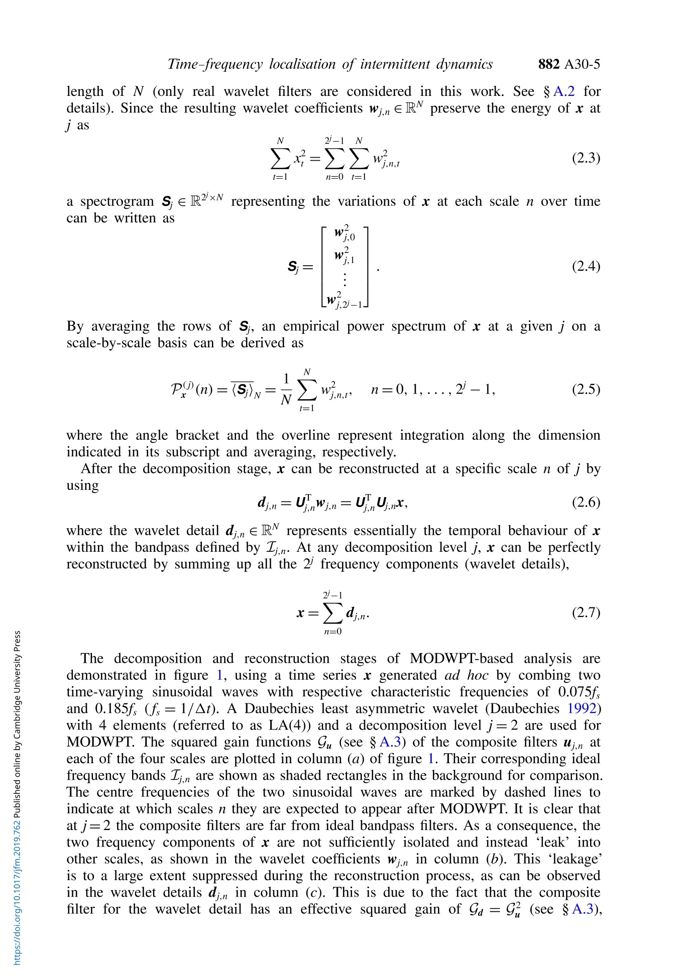
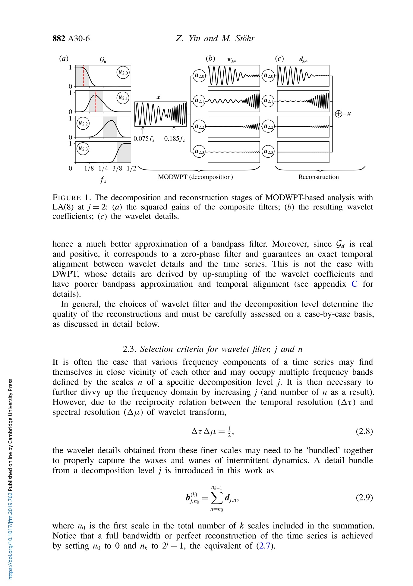
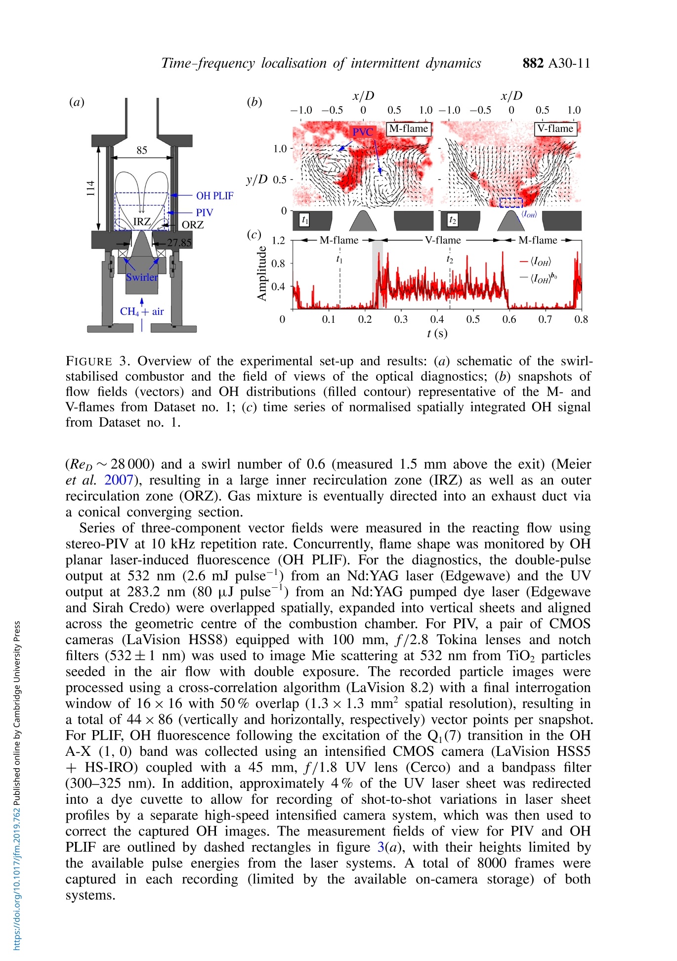
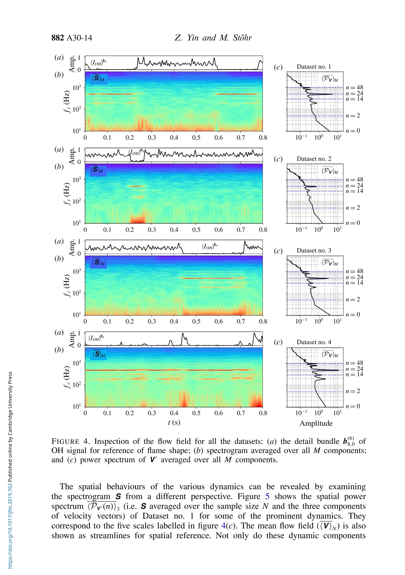
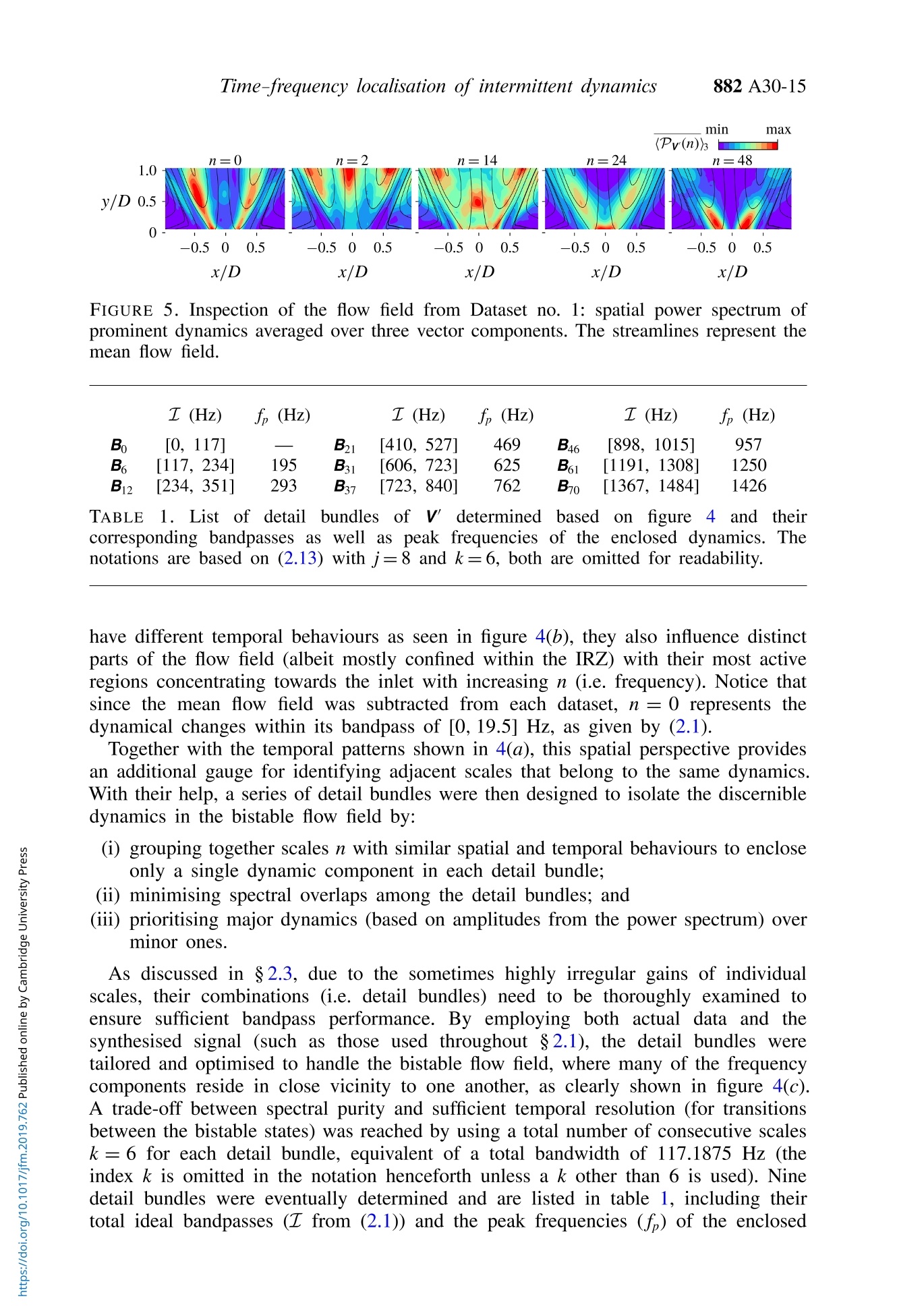
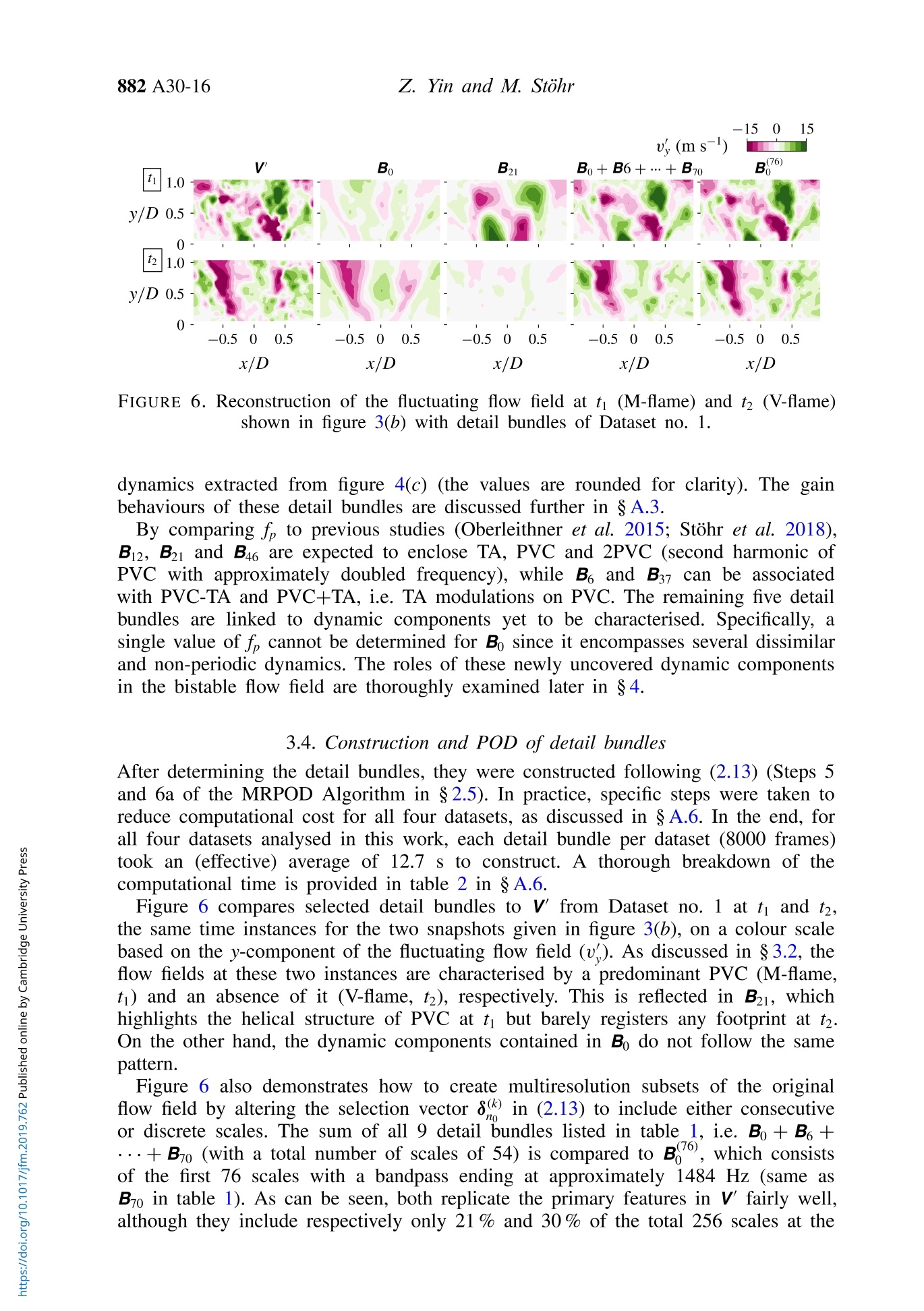
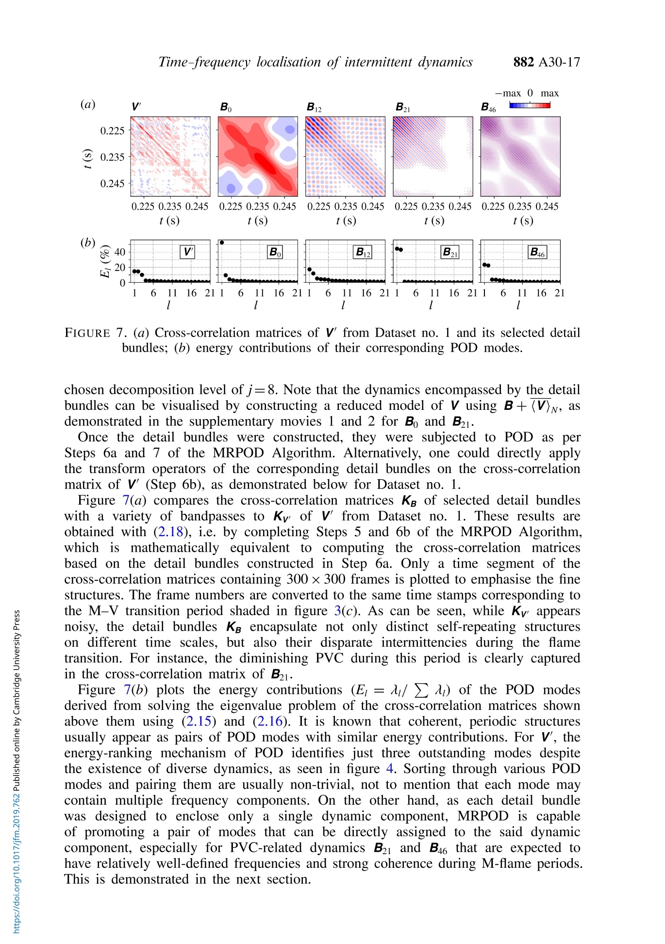
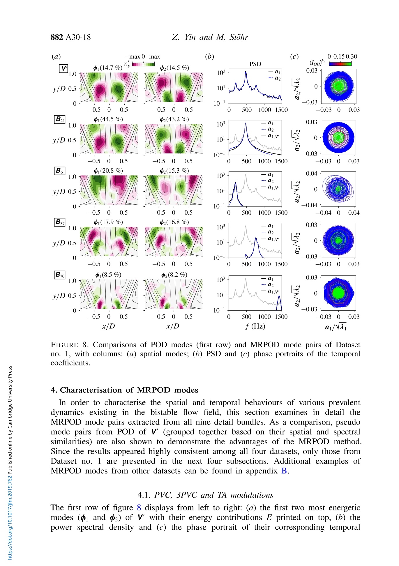
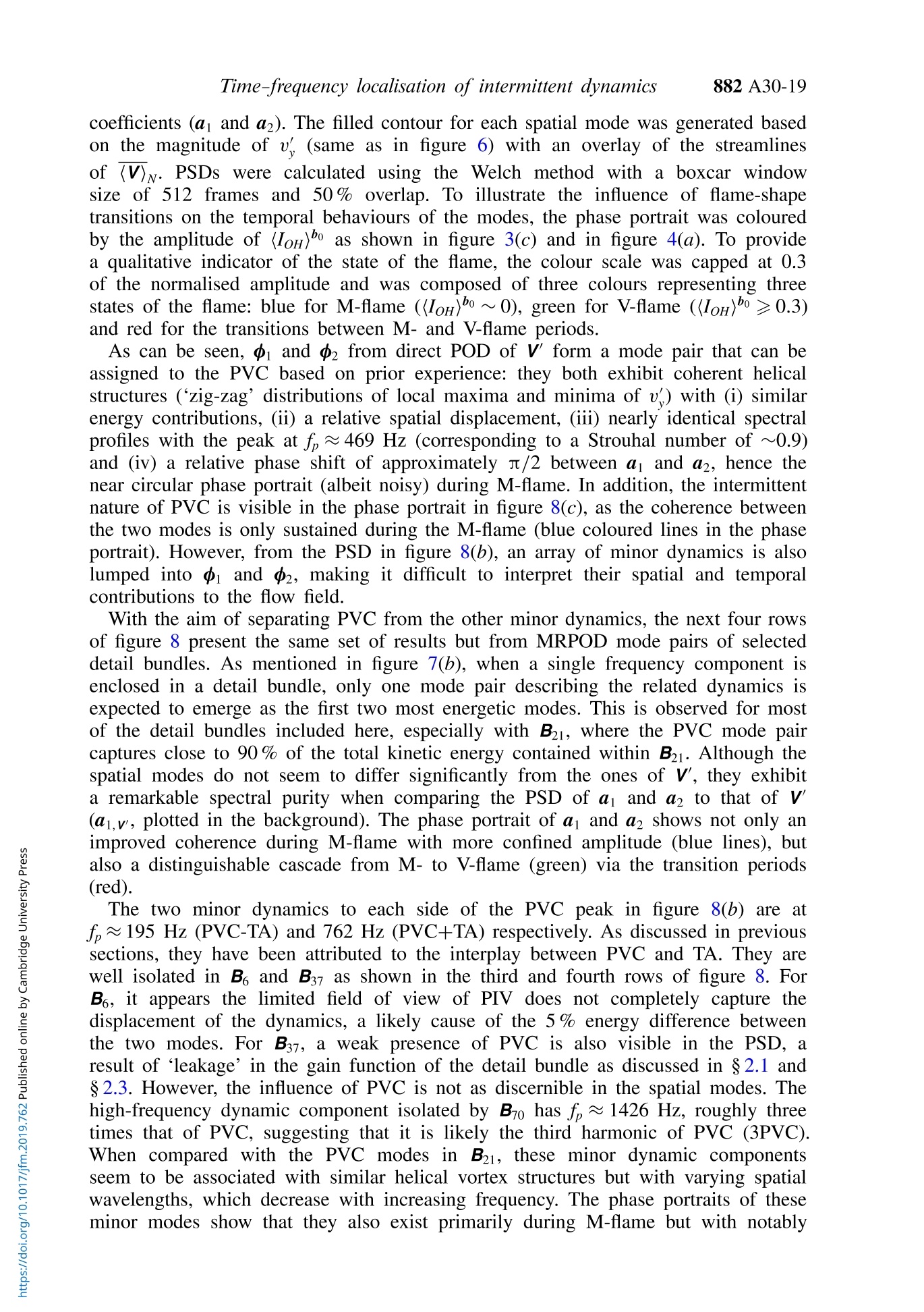
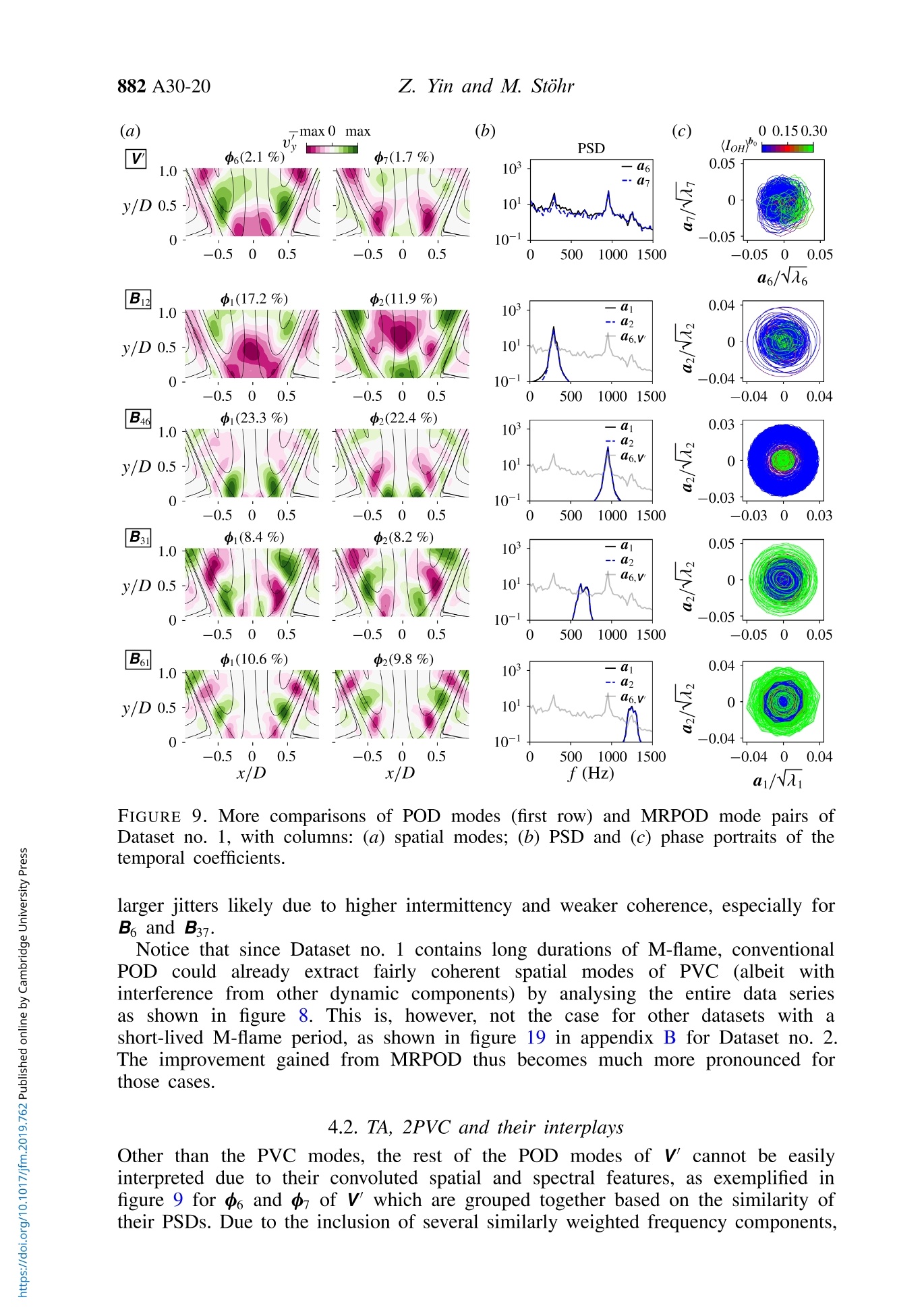
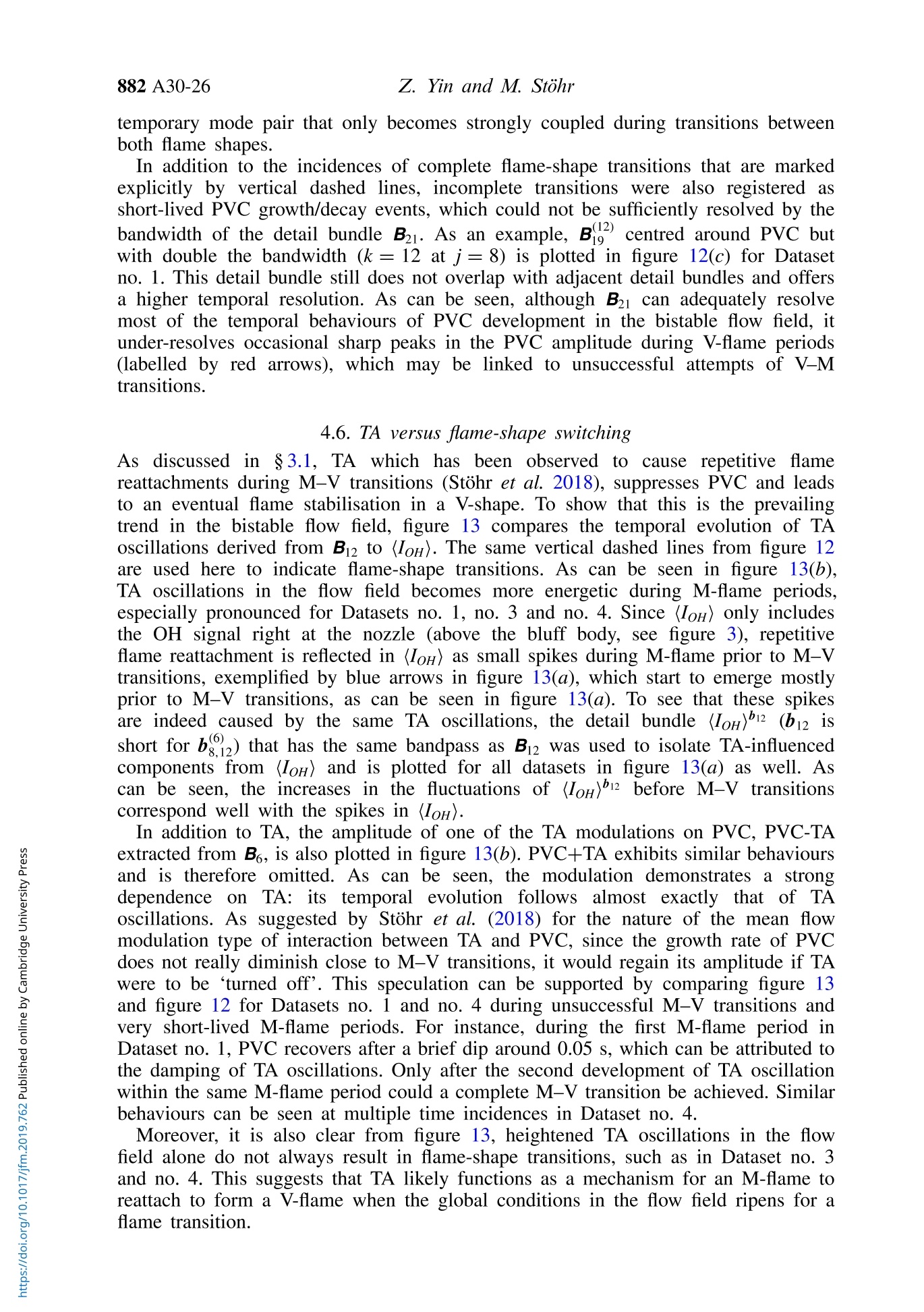
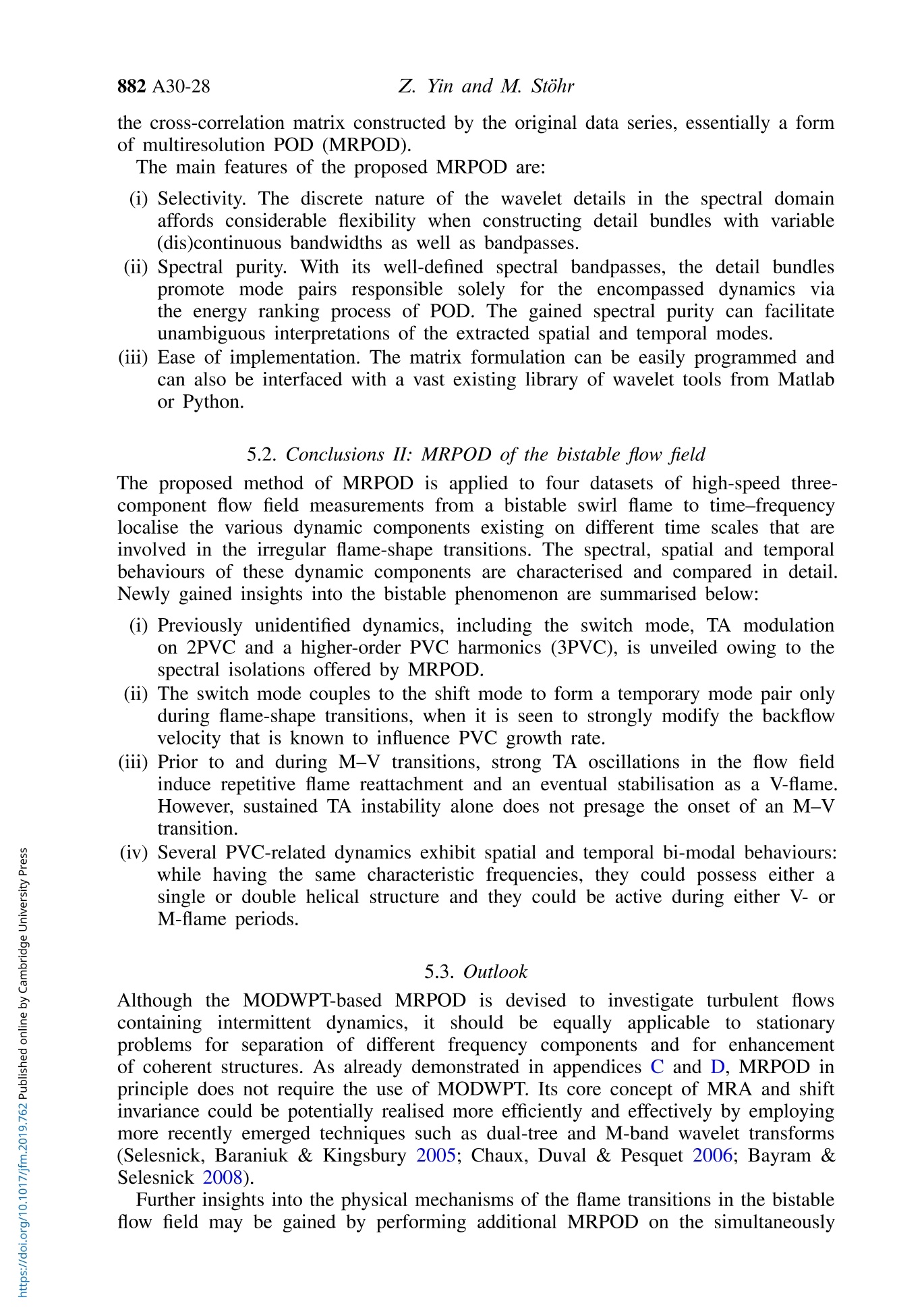
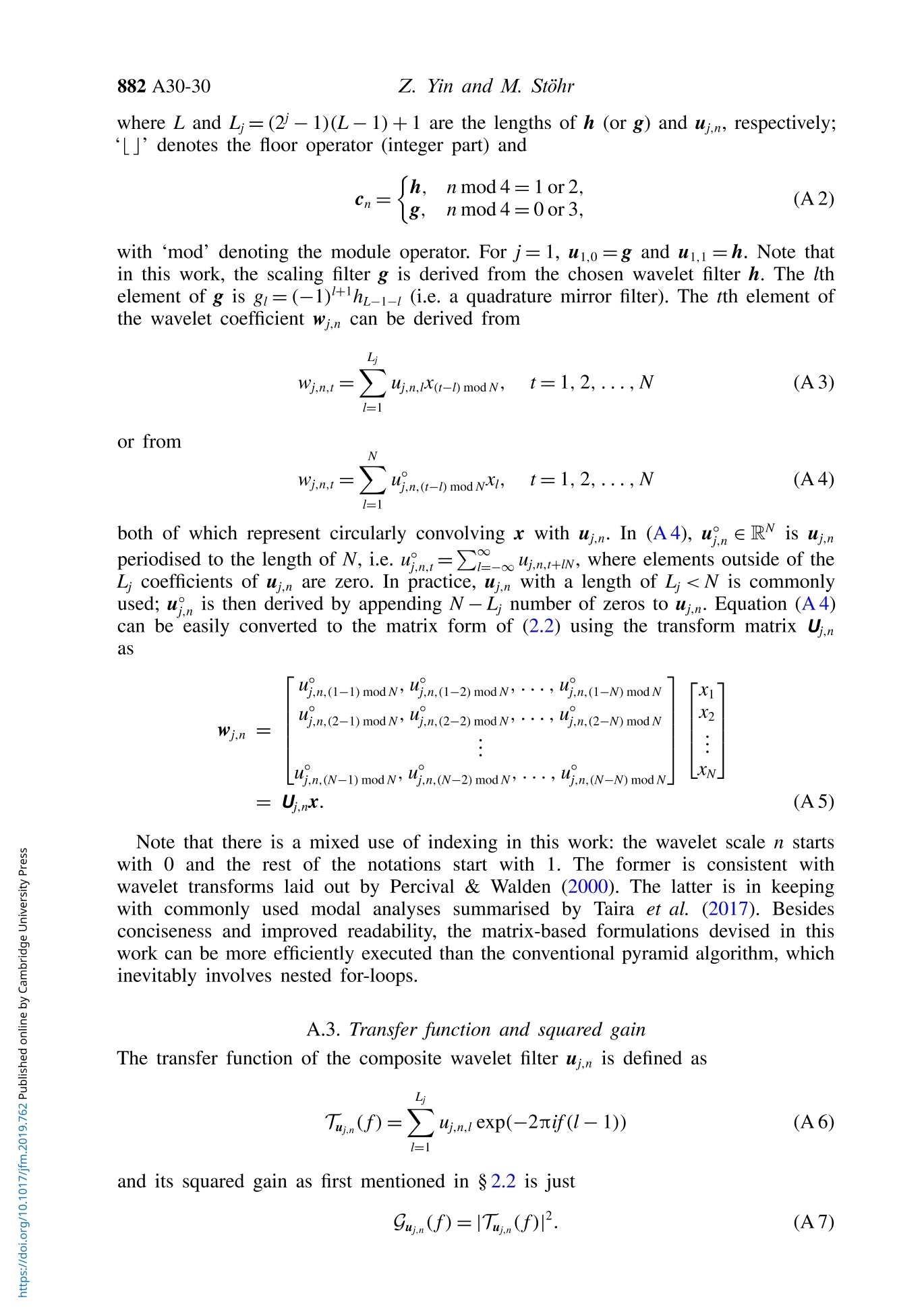
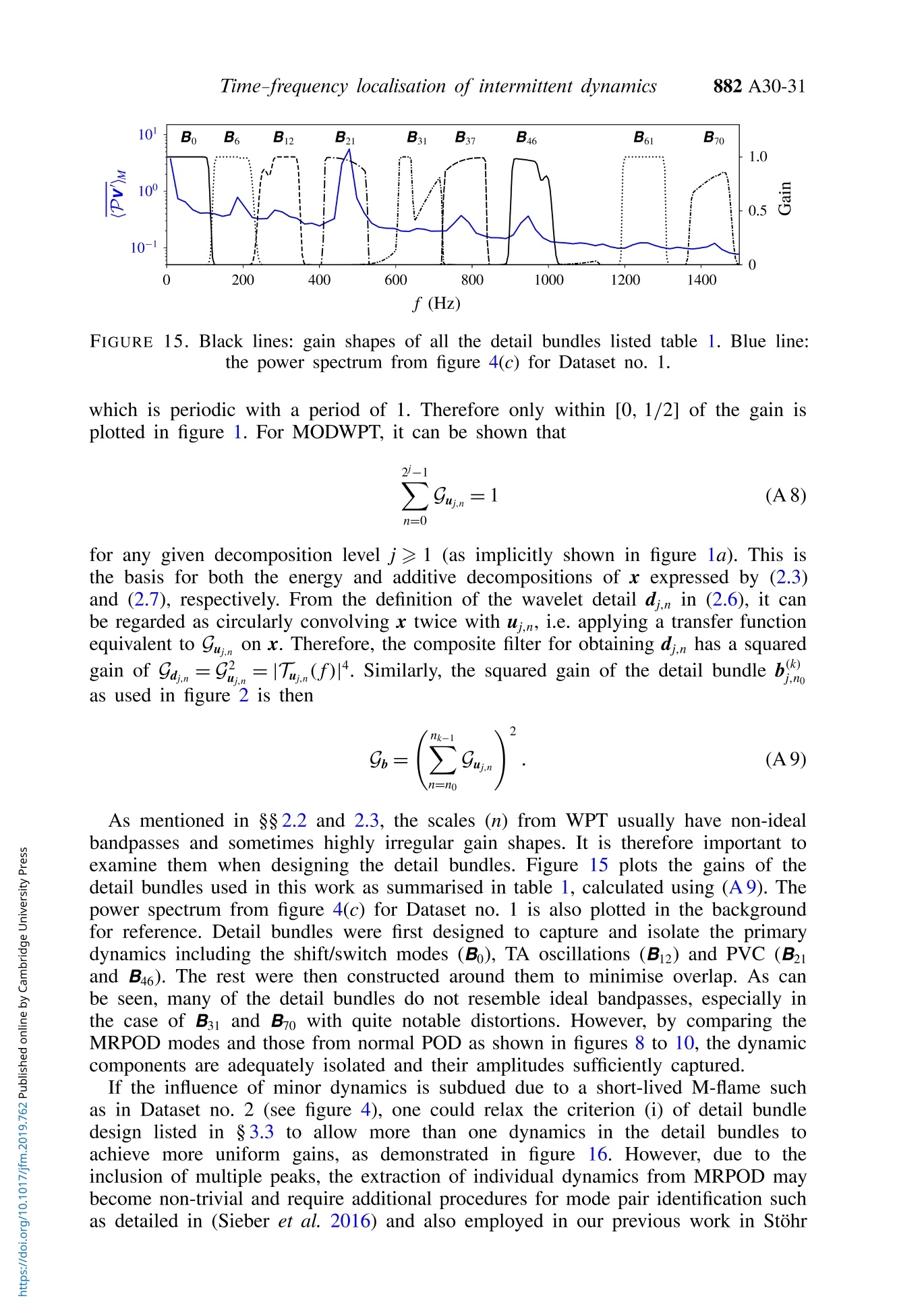
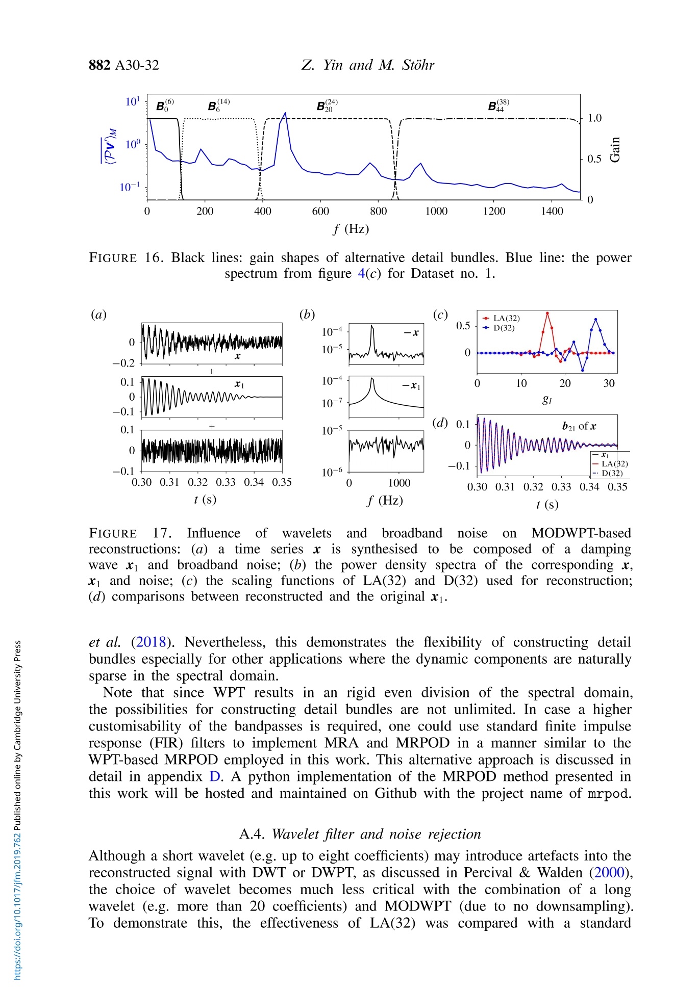
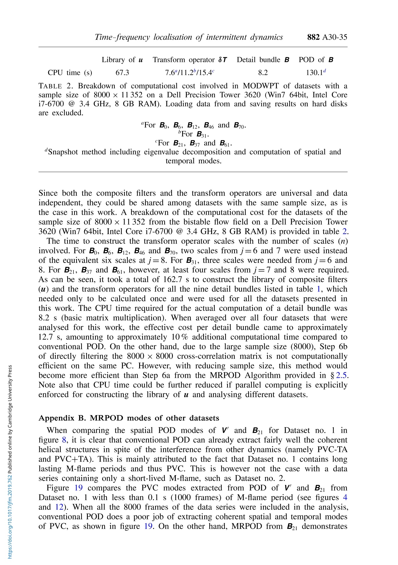
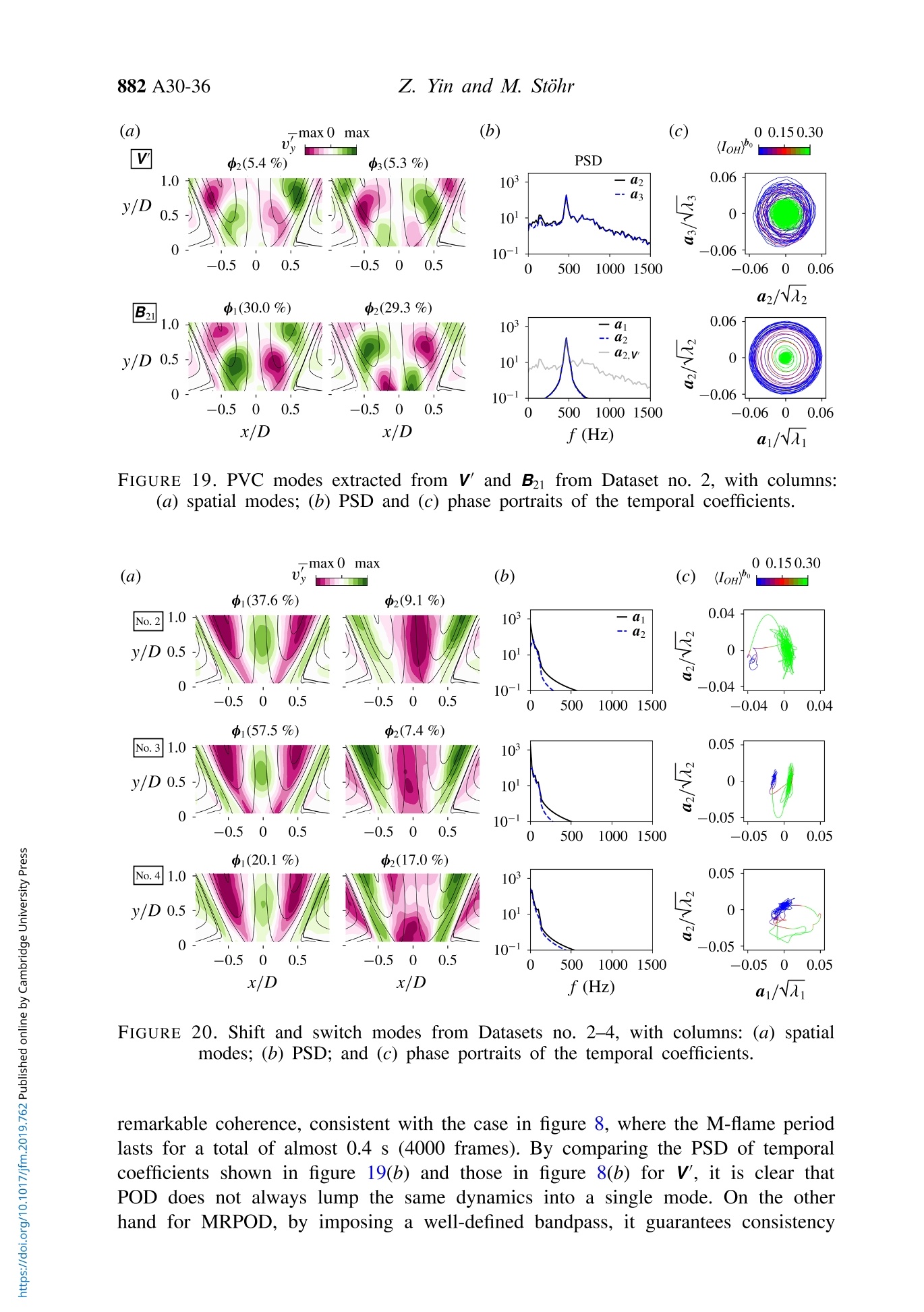
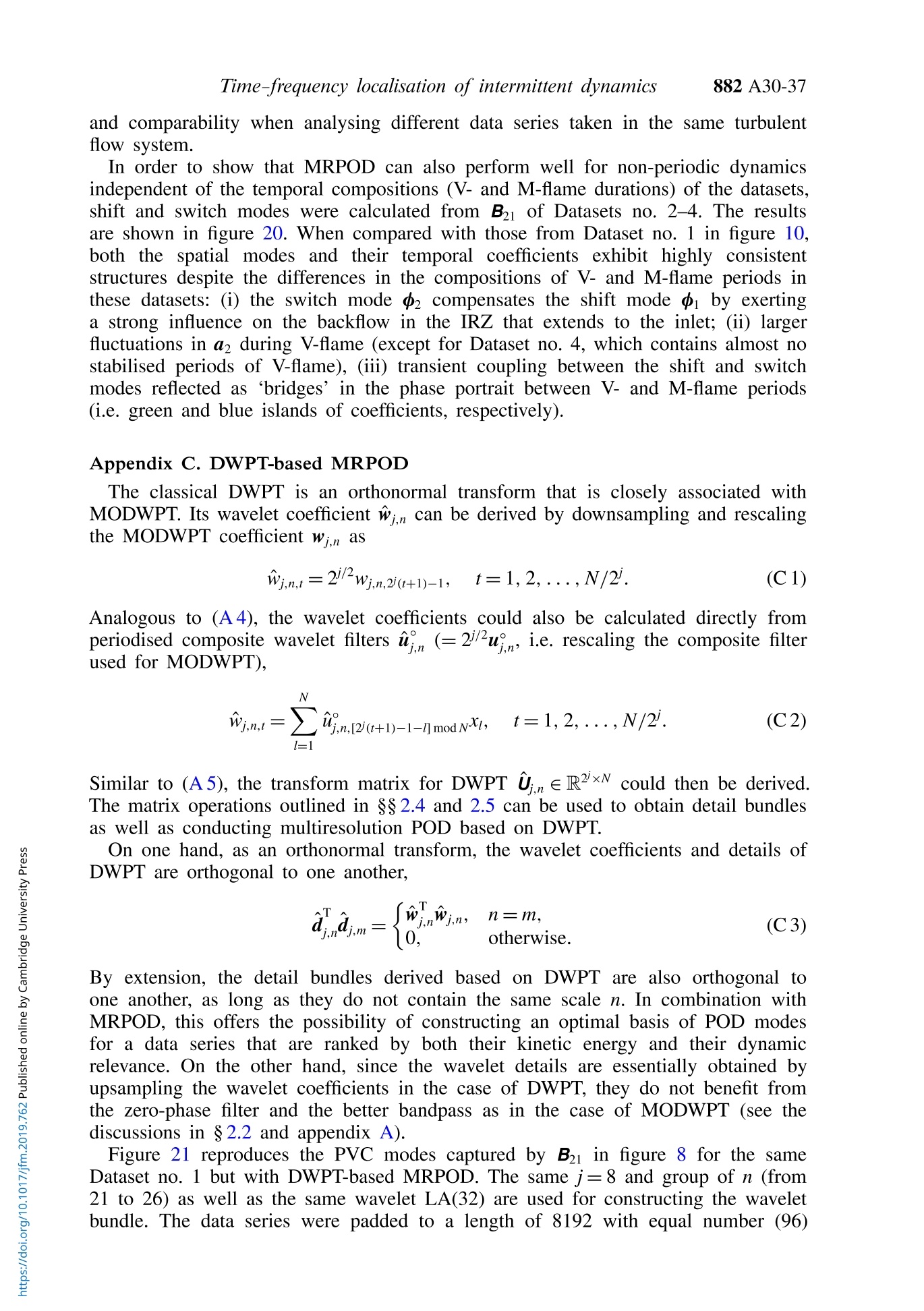
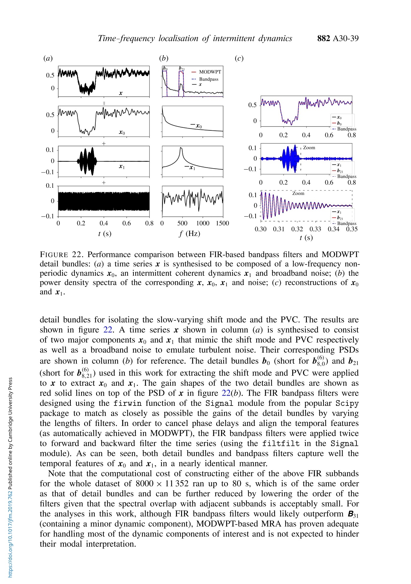
现代燃气轮机燃烧室内的湍流流动通常因为流体动力学和声学不稳定性以及火焰抬起、回流和双稳定性等非周期性动力学而表现出周期性振荡。此外，在完全发展的燃烧不稳定性之前，可能还会出现随机燃烧噪声和间歇性高幅度振荡爆发。这些现象可能同时出现在广泛的时间尺度上，并且也可能相互作用。由于火焰释放的热量变化会妨碍燃烧室的稳定、低排放运行，因此这些不稳定性的机理和控制在过去几十年中得到了密集的研究。具体来说，在旋流稳定的燃烧器中经常遇到的双稳态现象近年来受到了关注，火焰不规则地交替出现抬起的M形和附着的圆锥形V形。火焰形态的转变通常在几十毫秒内发生，并可能导致局部温度的急剧波动，从而导致不良情况，如热声脉动的突然增加或燃烧室的热应力。因此，深入理解这种双稳态现象对改进燃烧室设计至关重要。 为此，在一个基于工业设计的大气旋流稳定燃气轮机模型燃烧室中，建立了一个双稳态案例，该燃烧室已经得到了广泛的研究。该案例采用了高速光学诊断技术，包括同时粒子图像测速仪（PIV）和平面激光诱导荧光（OH PLIF）（Oberleithner等人，2015; Stöhr等人，2018）以及同时使用热测荧光粉的OH PLIF和表面测温法（Yin，Nau和Meier，2017）882 A30-1J. Fluid Mech. (2020)， vol. 882， A30.C The Author(s) 2019 z. Yin and M. Stohr882 A30-2 This is an Open Access article， distributed under the terms of the Creative Commons Attribution licence (h tt p：//creativecommons.o rg /licenses/b y /4.0/)， which permi ts unrest r icted re-use， distribution， and reproduction in any medium， provided the original work i s properly cited. doi：10.1017/jfm.2019.762 Time-frequency localisation of intermittent dynamics in a bistable turbulent swirl flame Zhiyao Yinl t and Michael Stohr l Institute of Combustion Technology， German Aerospace Center (DLR)， 70569 Stuttgar t ， Germany (Received 19 February 2019； revised 8 July 2019； accepted 11 September 2019) This work examines the complex flow field in a bistable turbulent swirl flame， where the flame alternates irregularly between a lifted-off M-shape and an attached V-shape.The flow field consists of various types of intermittent dynamics due to flame-shape switching that occur on different time scales. In order to properly identify， separate and temporally resolve these dynamic components， a novel method of multiresolution proper orthogonal decomposition (MRPOD) is developed by interfacing the maximum overlap discrete wavelet packet transform (MODWPT) of multidimensional data series with the conventional snapshot POD. Specific care is taken to select the wavelet filter， decomposition level and reconstruction bandwidth to achieve variable spectral bandpasses and adequate temporal resolutions.When applied to data series from high-speed three-component velocity field measurements in the bistable swirl fl ame，MRPOD is capable of isolating frequency components that are usually lumped i nto a single POD mode， with enhanced spatial/temporal coherence for even weak and highly intermittent dynamics. Owing to the i mproved spectral purity， a series of previously unknown dynamics is uncovered alongside well-characterised instabilities such as the precessing vortex core (PVC) and thermoacoustic (TA) instabilities. In particular， a non-periodic switch mode is found to couple with the previously identified shi f t mode only during flame-shape transitions， with pronounced modi f ications on the backflow and near the inlet of the combustor， a region known to i nfluence the growth rate of PVC. TA osci l lations are seen to drive repetitive flame reattachment during M-V transitions that eventually sett l es into a V-flame. But sustained high TA amplitudes alone do not appear to necessarily presage the onset of such a transition. Additional higher-order harmonics of PVC and evidence of TA modulations on PVC dynamics are uncovered， which also exhibit bi-modal behaviours： while maintaining their characteristic f requencies ， these instabilities could attain either a single or double helical structure and are only active during either V- or M-flame periods. Key words： combustion， computational methods， t urbulent reacting flows 1. Introduction Turbulent flows in modern gas turbine combustors often exhibit periodic osci l lations due to hydrodynamic and acoustic instabilities as well as non-periodic dynamics such as flame l ift-off， f lashback and bistability. In addition， stochastic combustion noise and intermittent bursts of high amplitude oscillations may occur prior to fully developed combustion i nstabilities (Gotoda et al. 2011； Nair， Thampi & Sujith 2014； Tony et al. 2015). These phenomena can occur simultaneously over wide-ranging time scales and may also interact with each other. The resulting variations of flame heat release impede the stable， low-emission operation of the combustor. Therefore， the mechanisms and control of these instabilities have been intensively studied during the past decades (Lieuwen & Yang 2005). Specifically， the bistability frequently encountered i n swirl-stabilised combustors has been under scrutiny in recent years (Fritsche， Furi & Boulouchos 2007； Biagioli，G uthe & Schuermans 2008； Hermeth et al. 2014： Guiberti et al. 2015： An et a 1.2016)， where the flame alternates in irregular successions between a lifted-off M-shape and an attached conical V-shape. The f lame-shape transitions usually take place over tens of milliseconds and could cause steep local temperature f luctuations， leading to undesirable situations such as sudden increase of thermoacoustic pulsations or thermal stress on the combustor chamber. A thorough understanding of this bistable phenomenon is therefore necessary for the improvement of combustor designs. For this purpose， a bistable case has been established in a well-studied atmospheric swirl-stabil i sed gas turbine model combustor based on an i ndustrial design (Roux et al. 2005； Meier et al . 2007； Franzelli et al. 2012； Steinberg， Arndt & Meier 2013). The case has been characterised by high-speed optical diagnostics including simultaneous particle image velocimetry (PIV) and planar laser-induced fluorescence of OH radicals (OH PLIF) (Oberleithner et al. 2015； Stohr et al. 2018) as well as simultaneous OH PLIF and surface thermometry employing t hermographic phosphors (Yin， Nau & Meier 2017). The resulting data series have most recently been analysed by Stohr et al. (2018) using spectral proper orthogonal decomposition (SPOD)(Sieber， Paschereit & Oberleithner 2016) and local linear stability analysis (LSA)(Rukes et al. 2017). An array of co-existing instabilities with diverse characteristic frequencies have been unveiled to underpin the flame-shape transitions： a shift mode representing the changes in the mean flow field， a helical processing vortex core (PVC)， a thermoacoustic (TA) axial pulsation in the inner recirculation zone (IRZ)of the combustor as well as instabil i ties linked to TA modulations on PVC. It has been demonstrated that PVC provides an unsteady stagnation point in the IRZ for stabilising of the M-flame. During an M-V transition， the development of TA instability suppresses PVC， leading to the destabilisation of the M-flame and i tsreattachment to the combustor inlet to form a V-flame. On the other hand， as the flame undergoes a V-M transi t ion， PVC is re-i nitiated and self-amplified， followed by re-establishment of the stagnation point in the IRZ and flame li f t-off. The non-periodic switching between the flame shapes is also accompanied by abrupt changes in the flow field， with transient and intermittent behaviours in normally coherent and periodic instabilities l ike PVC and TA. Data-driven modal decomposition methods such as POD (Lumley 1967； Sirovich 1987)and dynamic mode decomposition (DMD) (Rowley et al. 2009； Schmid 22010)have been implemented most commonly to extract periodic， coherent structures in turbulent f lows (Taira et al.2017). In their most b basic forms， however， their applicability to problems such as the bistable flame ishindered due too their inadequacies at identifying and separating intermittent dynamic components， which may possess similar spatial structures but which occur on a multitude of time scales.Spectral POD methods outlined by Sieber et al. (2016) and Towne， Schmidt &Colonius (2018)) provide additional ranking of the energetic modes according to their dynamic relevance but lack built-in mechanisms for separating closely packed frequency components and/or localising discontinuities i n the t emporal behaviours of the extracted modes. A variant of DMD that extracts time coefficients based on dynamic modes (Alenius 2014； Premchand et al. 2019) is capable of capturing temporal disruptions in coherent structures with well-defined frequencies Sbut t：is not suitable for handling t he non-periodic dynamics that governs the flame-shape switching. On the other hand， multiresolution analysis (MRA) based on discrete wavelet transform (DWT) (Mallat 1989) enables the expression of a time series as the sum of distinct components related to its variations on different time scales. Non-periodic and unsteady dynamics often rejected by Fourier analysis is preserved in MRA.Besides direct implementation of MRA on data series acquired i n turbulent flows (Ruppert-Felsot， Farge & Pet i tjeans 2009； Indrusiak & Moller 2011； Rinoshika &Omori 22011； Mancinelli et al. 2017； Kim et al. 2018)， the concept of MRA has 2016)a Buchlin 2019) that can potentially overcome the shortcomings of conventional modal analyses when treating complex dynamic systems. To further the understanding of the bistable phenomenon， this work proposes a novel approach to combine POD with wavelet-based MRA for deriving unambiguous modal descriptions of i ntermittent dynamics from the high-speed experimental data series obtained in the bistable flame.Instead of using DWT that offers limited， scale-dependent spectral resolutions， discrete vavelet packet transform (DWPT) (Coifman et al. 1994) was favoured for its larger basis of wavelet coefficients that allows a more f lexible time-frequency decomposition of the time series. Specifically， a shift-invariant version of DWPT， termed maximum overlap DWPT (MODWPT) (Percival & Guttorp 1994； Percival & Walden 2000)， is generalised into matrix forms to handle multidimensional data series. Care i s taken to select the wavelet filter and decomposition levels to achieve a desired balance between temporal and spectral resolutions. When interfaced with the conventional snapshot POD， it is shown that the method devised in this work attains the principle of a multiresolution POD (MRPOD). The enhanced capability of MRPOD in thea nalysis of complex unsteady turbulent flows is then demonstrated by newly gained insights into the bistable phenomenon. The paper is organised as follows： in $2， an overview is first given on the fundamentals of MODWPT of time series. A set of selection criteria are then provided for wavelet filters and decomposition levels. A generalised formulation i s subsequently derived to achieve efficient computation and to facilitate interfacing with snapshot POD. In S 3， MRPOD is applied to measured data series of the flow field in the bistable flame to extract modal descriptions of the data series within specific bandpasses in the spectral domain. In S 4， MRPOD modes are characterised and compared with POD modes for different frequency components. New f indings regarding the bistable flow field are discussed in detail. In 5， the results from t his work are summarised with an outlook on potential improvements and applications of the method of MRPOD presented in this work. 2. MODWPT-based modal analysis of time series The proposed approach seeks to facilitate a generalised implementation of wavelet packet transform (WPT) for handling time series of diverse dimensions. Since there exists a large variety of wavelet transforms and wavelet filters t hat can be used to perform a WPT， the choices are made based on the following criteria： (i) dynamics at various frequencies can be identified and adequately isolated， and (ii) abrupt changes in t heir temporal behaviours must be properly resolved and align perfectly with the original data series such that they can be correctly correlated in time. Before delving into the generalisation of the WPT method， this section begins with a brief introduction of DWPT and the rationale for choosing its shift-invariant version，namely the MODWPT. 2.1. Shift-invariant DWPT Generally speaking， DWPT carries out a time-frequency decomposition of a time series by projecting i t onto an orthonormal basis of wavelet filters， which is constructed by dilation and translation of a single wavelet function. Each of the resulting wavelet coefficients can be localised to a particular frequency/time interval.The time series can then be reconstructed based on the wavelet coefficients to allow for the analysis of its various frequency components separately. Since DWPT essentially expands upon a standard DWT by decomposing not only the scaling coefficients but also the wavelet coefficients at each decomposition level， its wavelet coefficients afford a higher flexibility and selectivity during reconstructions of the time series when compared to a DWT-based MRA (that can be viewed as a subset of DWPT-based reconstruction， see s A.1). Unlike DWPT， shift-invariant WPT such as MODWPT (similar variants i nclude undecimated (Shensa 1 on I verman 1995) DWPTs) is well defined for arbitrary sample sizes and is insensitive to the choice of the starting point in the time series. Moreover， MODWPT can offer higher spectral isolation during the reconstruction process， which becomes especially beneficial for handling time series laden with highly intermittent dynamic components that are densely packed in the spectral domain， as achieves these advantages at the expense of orthonormality， i t sti l l retains the ability to form an exact analysis of variance and a perfect reconstruction of the time series.Details are presented below. 2.2. Decomposition and reconstruction of time series The classical pyramid algorithm for MODWPT is illustrated in S A.1and is detailed in Percival & Walden (2000). This work opts for a composite filter approach that simplifies the matrix formulation given later in s 2.4 and offers a higher computational efficiency. For MODWPT of a time series x=[x1， X2， ...， xv]Te Ry， at each decomposition level j≥ 1， the frequency domain is divided equally into 2 s s c c a ales，with each scale n corresponding to a frequency bandpass of where At is the time step between two sampling points. The decomposition ofx using MODWPT at a specific scale n of j can be expressed as： The transform matrix U，ne RNxNis formed by time shifting row vectors of the composite wavelet filter uj，n constructed via filter cascade and periodised to the length of N (only real wavelet filters are considered in this work. See A .2 for details). Since the resulting wavelet coefficients WnR~preserve the energy of x at j as a spectrogram S，e R 2xN representing the variations of x at each scale n over t ime can be written as (2.4) By averaging the rows of S， an empirical power spectrum of x at a given j on a scale-by-scale basis can be derived as where the angle bracket and the overline represent integration along the dimension indicated in its subscript and averaging， respectively. After the decomposition stage， x can be reconstructed at a specific scale n of j by using where the wavelet detail djn e R~ represents essentially t he t emporal behaviour of x within the bandpass defined by Z，n. At any decomposition level j， x can be perfectly reconstructed by summing up all the 2 frequency components (wavelet details)， he decomposition and reconstruction stages of MODWPT-based analysis are d l e e r monstrated in figure 1， using a time series x generated ad hoc by combing two time-varying sinusoidal waves with respective characteristic frequencies of 0.075fs and 0.185fs (fs=1/At). A Daubechies least asymmetric wavelet (Daubechies 1992)with 4 elements (referred to as LA(4)) and a decomposition level j=2 are used for MODWPT . The squared gain functions Gu (see 8A.3) of the composite filters uj，n at each of the four scales are plotted in column (a) of figure 1. Their corresponding ideal frequency bands L，n are shown as shaded rectangles i n the background for comparison.The centre frequencies of the two sinusoidal waves are marked by dashed lines to indicate at which scales n they are expected to appear after MODWPT. It is clear that at j=2 the composite filters are far from ideal bandpass filters. As a consequence， the two frequency components of x are not sufficiently isolated and instead ‘leak’ into other scales， as shown i n the wavelet coefficients Wj，n in column (b). This ‘leakage’is to a large extent suppressed during the reconstruction process， as can be observed in the wavelet details dj，n in column (C). This is due to the fact that the composite filter for the wavelet detail has an effective squared gain of Ga=9 (see 8A.3)， FIGURE 1. The decomposition and reconstruction stages of MODWPT-based analysis with LA(8) at j=2： (a) the squared gains of the composite filters； (b) the resulting wavelet coefficients； (c) the wavelet details. hence a much better approximation of a bandpass filter. Moreover， since Ga is real and positive， it corresponds to a zero-phase filter and guarantees an exact temporal alignment between wavelet details and the t ime series. This is not the case with DWPT， whose detailsare derived by up-sampling of the wavelet coefficients and have poorer bandpass a approximation and temporal alignment (see appendix C for detai l s). In general， the choices of wavelet filter and the decomposition level determine the quality of the reconstructions and must be carefully assessed on a case-by-case basis，as discussed in detail below. 2.3. Selection criteria for wavelet filter， j and n It is often the case that various frequency components of a time series may f ind themselves in close vicinity of each other and may occupy multiple f requency bands defined by the scales n of a specific decomposition level j. It is then necessary to further divvy up the frequency domain by increasing j (and number of n as a result).However， due to the reciprocity relation between the temporal resolution (At) and spectral resolution (Au) of wavelet transform， the wavelet details obtained from these finer scales may need to be ‘bundled’ together to properly capture the waxes and wanes of intermittent dynamics. A detail bundle from a decomposition level j is introduced in t his work as where no is the first scale in the total number of k scales included i n the summation.Notice that a full bandwidth or perfect reconstruction of the time series is achieved by setting no to 0 and n to 2i -1， the equivalent of (2.7). FIGURE 2. Effects of wavelet size and reconstruction scales on the detail bundles： (a)the squared gain function corresponding to the three bundles compared to the normalised PSD of the synthesised time series y； (b-d) comparisons between reconstructed and the original time series. The size of the wavelet filter influences the squared gain function in a similar manner as dictated by (2.8)： the larger i t is the better i ts approximation of a bandpass filter. This comes with the caveat that the computational burden of MODWPT scales with the filter size and the resulting details may become more sensitive to boundary conditions of the time series (see A.5). As pointed out by Mouri et al. (1999)，turbulent statistics are largely independent of the choice of t he wavelets. The specific type of wavelet filter plays a lesser role for MODWPT， especially when a large filter is used， as shown in A.4. Among the most commonly used wavelet filters， this work has chosen the Daubechies wavelets as they have been widely adopted in turbulent flow applications (Indrusiak & Moller 2011； Rinoshika & Omori 2011； Mancinelli et al. 2017). Detailed performance comparisons of different wavelets are included in S A.4. Figure 2 demonstrates the effects of wavelet size and reconstruction scales on the detail bundles using another synthesised time series y (black l i nes)， whose normal i sed power spectral density (PSD) is plotted in figure 2(a). A decomposition l evel of j=8 is used to divide the frequency domain into 256 bands to allow for a sufficient amount of flexibility in constructing detail bundles to contain the frequency features within t heir bandpasses. Three detail bundles are compared here： (i) b21 with LA(8)(blue lines)， (ii) b23 with LA(32) (green l ines) and (iii) bs21 with LA(32) (red lines).Their corresponding squared gain functions G， are plotted in figure 2(a). As can be seen， the short wavelet filter of bundle (i) provides insufficient gain around the target frequency with undesirable gains in other bands， causing bundle (i) to notably miss the amplitude of y as shown in figure 2(b). Wi t h a much longer wavelet filter， bundle (ii) is able to spectrally isolate y but fails at resolving its fast decay due to the narrow total bandpass， as illustrated in f igure 2(c). On the other hand， with a combination of a long wavelet filter and an adequate bandwidth， bundle (iii) can well reproduce the magnitude as well as the temporal behaviour of y as evident in figure 2(d). It should be noted t hat， at higher decomposition levels， the gains of the i ndividual scales tend to deviate significantly from ideal bandpasses and become highly i r regular. I t is therefore important to examine the gain shapes when designing detail bundles， as discussed in detail i n 8A.3. To summarise， the choices of decomposition level， wavelet filter and reconstruction scales depend primarily on (i) the spectral resolution necessary for separating the target frequency components and (i i) the temporal resolution needed for resolving the intermittencies. In addition， the best basis algorithm (Coifman & Wickerhauser 1992)designed for DWPT can be used as an initial guidance for choosing the decomposition level j. 2.4. Generalisation to multidimensional data arrays The approach outlined in ǒ 2.2 is generalised to handle data arrays with a dimension of NxM，×M；×..×M， with N being the sample size in time. Let x； represent the time series obtained at an index i that spans all components n，s，...，5(other than time) of the data array. The data series can be arranged into a matrix XeRNxM as where M=M，×Mg ×.×M.. This is equivalent to reshaping the multidimensional data array by collapsing all non-time dimensions into row vectors and stacking them along the time axis. The MODWPT of X at a scale n of a decomposition level j can be expressed as where W e RNxM contains the wavelet coefficients wjn defined by (2.2) at all t he indices i. Similarly the wavelet details matrix DnERNM can be obtained based on (2.6) Finally， the detail bundles Be RAxM can be formulated as with the elements 8n of the row vector 8(k) e R" controlling the bandpass of the detail bundle and which is defined as Also recognise that the transform operator e R2/XNXNis independent of the c ontents of X and can be constructed a priori based on a chosen wavelet function，decomposition level j and the time dimension of the data series N. Following (2.7)，x can then be perfectly recovered by sett i ng all 8， to 1. In addition， each wavelet detail can be viewed as a detail bundle with k=1. When compared with the classical DWT-based MRA， WPT such as MODWPT offers a much larger basis of wavelet coefficients for reconstructing the time series within refined and variable bandpasses.The approximation (or smooth’) and details of a DWT-based MRA can also be readily computed based on (2.7)， by assigning an appropriate 8， to 1 (or 0) to achieve varying time resolutions (scales). Notice that the definition of the detail bundles given in (2.13) does not require the k number of scales n to be in sequence. This allows for grouping together of the discontinuous frequency bands during reconstruction for selective filtering of the time series. In practical implementation， (2.13) constitutes only a partial WPT (arbitrary disjoint dyadic decomposition) and can be efficiently computed by invoking f ewer equivalent parent scales from lower j levels to construct detail bundles at the target level， as further explained in S A.6. 2.5. Multiresolution POD With their wel l -defined spectral bandpasses， the detail bundles c ca an n be used 1as foundations for modal analyses to provide modal representations of the i solated dynamics of interest. This section formulates a multiresolution POD (MRPOD) that interfaces the wavelet detail bundles with conventional snapshot POD. Note that the indices j and n in the notation of the detail bundles are omitted in this section for readabil i ty. Following g t the classica al l d definition of snapshot POD (assuming N < M)， the igenvectors w=[y1，V2，...，Vv]eRNxN and eigenvalues A=diag(1，12，...，1v)e RNxN of the detail bundles B can be obtained by solving The spatial mode de RM can be written as where its temporal coefficient a eRY：is Alternatively， POD can also be applied directly to specific frequency components of X without explicitly constructing the detail bundles. This is made obvious by expanding the cross-correlation matrix Ke of B using (2.13) as This shows S that the POD of a specific detail bundle B constructed basedd on filtering X with 8T is equivalent to iteratively f i l tering the rows and columns of the cross-correlation matrix Kx of X with 8T (i.e. the two-dimensional discrete wavelet transform (2-D DWT) of Kx)， which naturally preserves the symmetry of the Hermitian matrix. This is analogous to the method proposed by Mendez et al.(2018)， where the filtering of Kx is achieved via 2-D DWT. Therefore， the notions of MRPOD and POD of detail bundles are used interchangeably in the following discussions. The core concept of MRPOD is s that， by simply altering the elements of the selection vector 8， POD can be performed either on the original data series or on a subset of the data series reconstructed within adjustable bandpasses that can even be discontinuous in the spectral domain. This can overcome one of the major drawbacks of POD： the inability to distinguish dynamics occurring at different time scales. It should be pointed out that the formulation of MRPOD in (2.15) does not necessari l y require the implementation of MODWPT. If the focus is placed rather on creating an z. Yin and M. Stohr orthogonal basis containing POD modes ranked by both kinetic energy and dynamic importance， the detail bundles can be constructed based on an orthonormal wavelet transform such as DWPT instead， as demonstrated in appendix C. If flexible frequency division and a highly controllable filter performance are needed， a generalised MRA using custom-designed bandpass filters can be adopted to conduct MRPOD (Mendez et al. 2019)， as discussed in appendix D. The ful 1l 1workflow for MRPOD i s summarised in the following step-by-step algorithm： Algorithm (MRPOD) 1. Rearrange the multidimensional dataset into a matrix Xe RNxM， as in (2.10). 2. Choose wavelet filter and decomposition level following $2.3. 3. Construct a l ibrary of composite f i lters with the chosen wavelet up to the desired maximal decomposition level， based on (A1). 4.(Optional ) Inspect the dataset and design detail bundles based on spectrograms constructed with wavelet coefficients， as in (2.4). 5. Construct transform operators 8()T for the detail bundles of interest， using the chosen wavelet filter， following (A5) and (2.13). 6. Carry out POD of detail bundles， take either of the following two steps： a. Compute detail bundles B with (2.13) and perform POD with (2.15). b. Directly filter croOSsSs--correlation matrix Kx of X with (2.18)) and solve its eigenvalue problem. 7. Compute modes with (2.16) and (2.17). Owing to the efficient matrix-based operations， the MODWPT-based MRPOD is computationally eff i cient for even large data volumes， as discussed in detail in $s 3.4and A.6. 3. MRPOD of the bistable reacting flow As the primary motivation of this aforementioned bistable turbulent swirl flame is analysed using the MRPOD approach described in $2. After an overview of the experiments， data series obtained from high-speed PIV is decomposed and reconstructed within different spectral bandpasses.The resulting detail bundles are then compared with each other based on their spatial and temporal POD modes. 3.1. Experimental set-up The experimental data analysed in this section were acquired by Stohr et al. (2018)from the widely researched PRECCINSTA combustor (Roux et al. 2005； Meier et al. 2007； Franzelli et al. 2012； Steinberg et al. 2013) operated at atmospheric pressure， with premixed methane (CH) and air at an equivalence ratio of 0.7， and thermal power of 20 kW. As shown schematically i n figure 3(a)， the combustor is composed of a cylindrical plenum with a diameter of 78 mm， a 12-vane swirl generator and a converging nozzle (D=27.85 mm) with a central conical bluff body.In addition， the combustor acoustics is decoupled from that of the gas delivery system by a sonic nozzle installed upstream of the plenum. The gas mixture is discharged into a combustion chamber (85× 85×114 mm’ with optical access through side walls made of quartz glass) at an average exit velocity (non-reacting) of 14.4m s-1 FIGURE 3. Overview of the experimental set-up and results： (a) schematic of the swirl-stabilised combustor and the field of views of the optical diagnostics； (b) snapshots of flow fields (vectors) and OH distributions (f illed contour) representative of the M- and V-flames from Dataset no. 1； (c) t i me series of normalised spatially i ntegrated OH signal from Dataset no. 1. (Rep~28000) and a swirl number of 0.6 (measured 1.5 mm above the exit) (Meier et al. 2007)， resulting in a large inner recirculation zone (IRZ) as well as an outer recirculation zone (ORZ). Gas mixture i s eventually directed into an exhaust duct via a conical converging section. Series of three-component vector fields were measured in the reacting f low using stereo-PIV at 10 kHz repet i tion rate. Concurrently， flame shape was monitored by OH planar laser-induced fluorescence (OH PLIF). For the diagnostics， the double-pulseoutput at 532 nm (2.6 mJ pulse -1) from an Nd：YAG laser (Edgewave) and the UV output at 283.2 nm (80 pJ pulse-) from an Nd：YAG pumped dye laser (Edgewave and Sirah Credo) were overlapped spatially， expanded i nto vertical sheets and aligned across the geometric centre of the combustion chamber. For PIV， a pair of CMOS cameras (LaVision HSS8) equipped with 100 mm， f/2.8 Tokina lenses and notch filters (532±1 nm) was used to image Mie scattering at 532 nm from TiO particles seeded in the air flow with double exposure. The recorded particle i mages were processed using a cross-correlation algorithm (LaVision 8.2) with a final interrogation window of 16 × 16 with 50 % overlap (1.3×1.3 mm²spatial resolution)， result i ng in a total of 44 ×86 (vertically and horizontally， respectively) vector points per snapshot.For PLIF， OH f luorescence following the excitation of the Q (7) transition i n the OH A-X (1，0) band was collected using an intensi f ied CMOS camera (LaVision HSS5+ HS-IRO) coupled with a 45 mm， f/1.8 UV lens (Cerco) and a bandpass fi l ter (300-325 nm). I n addi t ion， approximately 4% of the UV laser sheet was redirected into a dye cuvette to allow for recording of shot-to-shot variations i n laser sheet profiles by a separate high-speed i ntensified camera system， which was then used tocorrect the captured OH images. The measuremen t fields of view for PlV and OH PLIF are outlined by dashed rectangles in figure 3(a)， with their heights limited by the available pulse energies from the laser systems. A total of 8000 frames were captured in each recording (limited by the available on-camera storage) of 1both systems. z. Yin and M. Stohr 3.2. Overview of experimental results The connections between flame shapes and combustion stabilities as w well aass the mechanisms governing these transitions have been studied extensively in premixed swirl-stabilised combustors (Shanbhogue et al . 2016； Taamallah， Shanbhogue &Ghoniem 2016). A series of experimental surveys was conducted in the PRECCINSTA combustor by Oberleithner et al. (2015) to analyse the stabilisation mechanisms of swir l flame. It was observed that， at a given thermal power， t he flame could be stabi l ised in a lifted-off M-shape at leaner conditions with the presence of PVC and in an attached V-shape where PVC was suppressed when the equivalence ratio was increased. At certain intermediate equivalence ratios， bistable cases emerged where the f lame alternates non-periodically between a lifted-off M-shape and an attached V-Shape， such as at the operat i ng condition used in this work (described in $ 3.1).Figure 3(b) shows t he overlaid instantaneous flow field and OH distributions selected from Dataset no. 1 (a recording of 8000 frames or equivalently 0.8 s) to represent a typical M- and V-flame， respectively. The signature ‘zig-zag’vortex pattern of PVC is also visible in the flow field of the M-flame， but is absent during V-flame.The OH signal within a 10 mm by 4 mm region as outlined in t he V-flame in figure 3(b) above the bluff body is integrated to track the flame shapes. The result i ng，normalised time series of (Ion) (angle bracket denotes spatial integration) is plotted in figure 3(c). Time zero is set at the first frame of the recording， and the periods of the M- and V-flames are qualitatively labelled in figure 3(c). The respective t i me stamps of the two snapshots shown in figure 3(b) are marked as t and t2. As can be seen， the time series starts and ends with a V-flame and experiences two V-M and M-V transitions with a total of approximately 0.4 s residing in either bistable state.The f lame detachment and reattachment processes during V-M and M-V transitions (each occurs and completes within about 0.05 s) are captured in detail by overlaid distributions of OH PLIF and velocity vectors in the supplementary movies 1 and 2 are available online at https：//doi.org /10.1017/jfm.2019.762. In addition to Dataset no. 1， three other datasets with the same sample volume but which are composed of various constellations of M- and V-flame periods are analysed in the following sections. Following the previous studies， this work employs the MODWPT-based MRPOD to time-frequency localise all relevant intermittent dynamics i n the f low f ield of the bistable flame， with a focus on (i) providing unambiguous modal descriptions of known/unknown frequency components and (ii) seeking prevailing trends shared among different datasets consisted of varying durations of V- and M-flames. 3.3. Inspection of the flow field In order to determine all the relevant intermittent dynamics， an inspection of the (i )temporal and (ii) spatial behaviours of various frequency components in the bistable flow field was carried out by constructing spectrograms， i.e. Step 4 of the MRPOD Algorithm given at the end of $2.5. Specifically， each of the time series of measured flow field as exemplified in figure 3 (subtracted by its series mean) was first organised into an N× M matrix of V'=[u’，u，...，]， with an N of 8000 (snapshots) and M of 11352 (=3×44 ×86， i.e. total number of measured velocity components per snapshot). Based on a prel i minary examination of vector series extracted from different regions in the flow field following consideration of the spectral and temporal resolutions outlined in s 2.3， a decomposition level of j= 8 (i.e. 256 scales n) and the LA(32) filter were chosen to perform the MODWPT of V' using (2.11) and then to construct the spectrograms using (2.4). Note t hat the spectrogram S of each dataset has a dimension of 2×N× M (the index j is omitted in t he notations of the forthcoming discussion as it is kept the same). Results from all four datasets including Dataset no. 1 shown in figure 3 are presented in f igure 4. For each dataset， figure 4(b-c) shows the spectrogram (S)M (i.e. S e R2xNxM averaged over all M components) on a log colour scale (same for all datasets)and the empirical power spectrum (Pv)m of V’ averaged over all M coommppone generated using (2.4)， (2.5) and the wavelet coefficient matrices W.. The frequency axis in both plots corresponds to the centre frequency fe of each scale n. Note that for LA(32) and at j= 8， the phase shi f t in wavelet coefficients are not negligible 三 and need to be compensated for such that the coef f icients are aligned to the original data series in t ime (Percival & Walden 2000). While the spectrogram provides an overview of the temporal behaviours of various frequency components， the power spectrum compares their absolute amplitudes. Additionally， a detail bundle (Ion)bo of (Ion) with a bandpass of [0， 117.1875] Hz (bo is short for b) was derived using (2.9) to track only the states of the flames as well as the transitions between them，both of which occur on a fairly large time scale. Here (Ion)is shown together with (Ion) in f i gure 3(c) for Dataset no. 1 as an example and is plotted in f i gure 4(a) for reference of the bistable states. As can be seen in all four cases， the flow field consists of a l arge variety of dynamic components occuring over a wide spectral range， some of which are highly intermittent. When compared to (Ion)， it is clear t hat these frequency components do not always overlap in time： while the prominent peak at n=24， corresponding to PVC， appears to exist only during the M-flame， while others are more discernible during the V-flame (e.g. at n=2) or become especially exited during flame transitions (e.g. between n =0 and 2). The irregular and non-periodic nature of the bistable flame-shape switching is made obvious by comparing the datasets： t he durations of either V- or M-flame as well as the incidences of (in)complete flame-shape transitions vary drastically from dataset to dataset. For instance， while Dataset no. 2 exhibits only a brief period of M-f lame between 0.2 and 0.3 s， Dataset no. 4 is dominated almost entirely by an M-flame， which only switches into a V-flame towards the end of the recording. Despite such di f ferences， all the datasets share some common features： (i)a complete flame-shape transition (V-M or M-V) takes place within approximately 0.05 s， as pointed out in the discussions of figure 3(c)； and (ii) the same frequency components can be identi f ied in the spectrograms with consistent temporal behaviours with regard to the flame-shape indicator of (Ion)o， albeit with different magnitude，as shown in their corresponding power spectra. (Ion) Lwwwwww FIGURE 4. Inspection of the flow field for all the datasets： (a) the detail bundle b 品of OH signal for reference of flame shape； (b) spectrogram averaged over all M components；and (c) power spectrum of V’averaged over all M components. The spatial behaviours of the various dynamics can be revealed by examining the spectrogram s from a different perspective. Figure 5 shows the spatial power spectrum (Pv(n))3 (i.e. S averaged over the sample size N and the three components of velocity vectors) of Dataset no. 1 for some of the prominent dynamics. They correspond to the five scales labelled in figure 4(C). The mean flow field ((V)v) is also shown as streamlines for spatial reference. Not only do these dynamic components _ min max FIGURE 5. Inspection of the flow field from Dataset no. 1： spatial power spectrum of prominent dynamics averaged over three vector components. The streamlines represent the mean flow f ield. 工 (Hz) f， (Hz) z (Hz) f， (Hz) z (Hz) f， (Hz) Bo [O，117] B21 [410，527] 469 B46 [898，1015] 957 B6 [117，234] 195 B31 [606，723] 625 B61 [1191，1308] 1250 B12 [234，351] 293 B37 [723，840] 762 B70 [1367，1484] 1426 TABLE 1. List of detail bundles of V’ determined based on figure 4 and t heir corresponding bandpasses as well as peak frequencies of the enclosed dynamics. The notations are based on (2.13) with j=8 and k=6， both are omitted for readability. have different temporal behaviours as seen in f igure 4(b)， t hey also influence dist i nct parts of the flow field (albeit mostly confined within the IRZ) with their most active regions concentrating towards the inlet with increasing n (i .e. frequency). Notice that since the mean flow field was subtracted from each dataset， n = 0 represents the dynamical changes within its bandpass of [0， 19.5] Hz， as given by (2.1). Together with the temporal patterns shown in 4(a)， this spatial perspective provides an additional gauge for identifying adjacent scales t hat belong to the same dynamics.With their help， a series of detail bundles were then designed to isolate the discernible dynamics in the bistable flow field by： (i) grouping together scales n with similar spat i al and t emporal behaviours to enclose only a single dynamic component in each detail bundle； (ii) minimising spectral overlaps among the detail bundles； and (iii) prioritising major dynamics (based on amplitudes from the power spectrum) over minor ones. As discussed in $2.3， due to the sometimes highly irregular gains of i ndividual scales， their combinations (i.e. detail bundles) need to be thoroughly examined to ensure sufficient bandpass performance. By employing both actual data and the synthesised signal (such as those used throughout 2.1)， t he detail bundles were tailored and optimised to handle the bistable flow field， where many of the frequency components reside in close vicinity to one another， as clearly shown in figure 4(c).A trade-off between spectral purity and sufficient temporal resolution (for transitions between the bistable states) was reached by using a total number of consecutive scales k= 6 for each detail bundle， equivalent of a total bandwidth of 117.1875 Hz (the index k is omitted in the notation henceforth unless a k other than 6 i s us ed). Nine detail bundles were eventually determined and are l isted in t able 1， i ncluding their total ideal bandpasses (Z from (2.1)) and the peak frequencies (fp) of the enclosed FIGURE 6. Reconstruction of the fluctuating flow field at t (M-flame) and t2 (V-flame)shown in figure 3(b) with detail bundles of Dataset no. 1. dynamics extracted from figure 4(c) (the values are rounded for clarity). The gain behaviours of these detai l bundles are discussed further in ǒ A.3. By comparing f， to previous studies (Ober l eithner et al. 2015； Stohr et al. 2018)，B12， B21 and B46 are expected to enclose TA， PVC and 2PVC (second harmonic of PVC with approximately doubled frequency)， while B6 and B37 can be associated with PVC-TA and PVC+TA， i.e. TA modulations on PVC. The remaining five detail bundles are l i nked to dynamic components yet to be characterised. Speci f ically， a single value of f， cannot be determined for Bo since i t encompasses several dissimilar and non-periodic dynamics. The roles of these newly uncovered dynamic components in the bistable flow field are thoroughly examined later in 8 4. 3.4. Construction and POD of detail bundles After determining the detail bundles， they were constructed following (2.13) (Steps 5and 6a of the MRPOD Algorithm i n 2.5). In practice， specific steps were taken to reduce computational cost for all four datasets， as discussed in A.6. In t he end， for all four datasets analysed in this work， each detail bundle per dataset (8000 frames)took an (effective) average of 12.7 s to construct. A thorough breakdown of the computational time is provided in table 2 in 8A.6. Figure 6 compares selected detail bundles to V’ from Dataset no. 1 at t and t2，the same t ime instances for the two snapshots given i n f igure 3(b)， on a colour scale based on the y-component of t he fluctuating flow field (). As discussed in $ 3.2， the flow f i elds at these two instances are characterised by a predominant PVC (M-flame，ti) and an absence of it (V-flame， t2)， respectively. This is reflected in B21， which highlights the helical structure of PVC at t but barely registers any footprint at t 2.On the other hand， the dynamic components contained in Bo do not follow the same pattern. Figure 6 also demonstrates how to create multiresolution subsets of the original flow field by altering the selection vector 8(k) in (2.13) to include either consecutive or discrete scales. The sum of all 9 detail bundles listed in table 1， i.e. Bo+B6+...+ Bzo (with a total number of scales of 54) is compared to B， which consists of the first 76 scales with a bandpass ending at approximately 1484 Hz (same as B7o in table 1). As can be seen， both replicate the primary features in V’ fair l y well ，although they include respectively only 21% and 30 % of the total 256 scales at the FIGURE 7. (a) Cross-correlation matrices of V’ from Dataset no. 1 and its selected detail bundles； (b) energy contributions of their corresponding POD modes. chosen decomposition level of j=8. Note that t he dynamics encompassed by the detail bundles can be visualised by constructing a reduced model of V using B+(V)v， as demonstrated in the supplementary movies 1 and 2 for Bo and B21· Once the detail bundles were constructed， they were subjected to POD as per Steps 6a and 7 of the MRPOD Algorithm. Alternatively， one could directly apply the transform operators of the corresponding detail bundles on the cross-correlation matrix of V’ (Step 6b)， as demonstrated below for Dataset no. 1. Figure 7(a) compares the cross-correlation matrices Ke of selected detail bundles with a variety of bandpasses to Ky of V’ from Dataset no. 1. These results are obtained with (2.18)， i.e. by completing Steps 5 and 6b of the MRPOD Algorithm，whichi s s mathematically equivalent to computing the cross-correlation matrices based on the detail bundles constructed in Step 6a. Only a time segment of the cross-correlation matrices containing 300× 300 frames is plot t ed to emphasise the f i ne structures. The frame numbers are converted to t he same time stamps corresponding to the M-V transition period shaded in figure 3(c). As can be seen， while Ky appears noisy， the detail bundles Ke encapsulate not only distinct self-repeat i ng structures on different time scales， but also their disparate i ntermittencies during the flame transition. For instance， the diminishing PVC during this period is clearly captured in the cross-correlation matrix of B21· Figure 7(b) plots the energy contribut i ons (Ei=A/A ) of the POD modes derived from solving the eigenvalue problem of the cross-correlation matrices shown above them using (2.15) and (2.16). I t is known that coherent， periodic structures usually appear as pairs of POD modes with similar energy contributions. For V， the energy-ranking mechanism of POD ident i fies just three outstanding modes despite the existence of diverse dynamics， as seen in figure 4. Sorting through various POD modes and pairing them are usually non-trivial， not to mention that each mode may contain multiple frequency components. On the other hand， as each detail bundle was designed to enclose only a single dynamic component， MRPOD i s capableof promoting a pair of modes that can be directly assigned to the said dynamic component， especially for PVC-related dynamics B21 and B46 that are expected to have relatively well-defined frequencies and strong coherence during M-flame periods.This is demonstrated in the next section. FIGURE 8. Comparisons of POD modes (first row) and MRPOD mode pairs of Dataset no. 1， with columns： (a) spatial modes； (b) PSD and (c) phase portraits of the t emporal c oefficients. 4. Characterisation of MRPOD modes In order to characterise the spatial and temporal behaviours of various prevalent dynamics existing in the bistable f low f ield， this section examines i n detail the MRPOD mode pairs extracted from all nine detail bundles. As a comparison， pseudo mode pairs from POD of V’ (grouped together based on their spatial and spectral similarities) are also shown to demonstrate the advantages of the MRPOD method.Since the results appeared highly consistent among all four datasets， only those from Dataset no. 1 are presented in the next four subsections. Additional examples of MRPOD modes from other datasets can be found in appendix B. 4.1. PVC， 3PVC and TA modulations The first row of f igure 8 displays from left to right： (a) the first two most energetic modes ((i and p2) of V’ with their energy contributions E printed on top， (b) the power spectral density and (c) the phase portrait of their corresponding temporal coefficients (a and a2). The filled contour for each spat i al mode was generated based on the magnitude of u’ (same as in figure 6) with an overlay of the streamlines of (V)y. PSDs were calculated using the Welch method with a boxcar window size of 512 frames and 50% overlap. To il l ustrate the influence of flame-shape transitions on the temporal behaviours of the modes， the phase portrait was coloured by the amplitude of (Ion)o as shown in figure 3(c) and in f igure 4(a). To provide a qualitative indicator of the state of t he flame， the colour scale was capped at 0.3of the normalised amplitude and was composed of three colours representing three states of the flame： blue for M-flame ((Ion)bo~0)， green for V-flame ((Ion)bo≥ 0.3)and red for the transitions between M- and V-flame periods. As can be seen， pi and d2 from direct POD of V' form a mode pair that can be assigned to the PVC based on prior experience： they both exhibit coherent helical structures (‘zig-zag’distributions of local maxima and minima of u) with (i ) similar energy contributions， (ii) a relative spatial displacement， (iii ) nearly identical spectral profiles with the peak at fp~469 Hz (corresponding to a Strouhal number of ~0.9)and (iv) a relative phase shift of approximately n/2 between a and a2， hence the near circular phase portrait (albeit noisy) during M-flame. In addition， t he intermittent nature of PVC is visible in the phase portrait in figure 8(c)， as the coherence between the two modes is only sustained during the M-flame (blue coloured lines in the phase por t rait ). However， from the PSD in f i gure 8(b)， an array of minor dynamics i s also lumped into di and d2， making it difficult to interpret their spatial and temporal contributions to the f low field. With the aim of separating PVC from t he other minor dynamics， the next four rows of figure 8 present the same set of results but from MRPOD mode pairs of selected detail bundles. As mentioned in figure 7(b)， when a single frequency component is enclosed in a detail bundle， only one mode pair describing the related dynamics is expected to emerge as the f i rst two most energetic modes. This is observed for most of the detail bundles included here， especially with B21， where the PVC mode pair captures close to 90 % of the total kinetic energy contained within B21. Although the spatial modes do not seem to differ significantly from the ones of V'， they exhibit a remarkable spectral purity when comparing the PSD of a and a2 to that of V'(a1，w， plotted in the background). The phase portrait of a and a2 shows not only an improved coherence during M-flame wi t h more confined amplitude (blue lines)， but also a distinguishable cascade from M- to V-flame (green) via the transition periods (red). The two minor dynamics to each side of the PVC peak in figure 8(b) are at f，~ 195 Hz (PVC-TA) and 762 Hz (PVC+TA) respectively. As discussed i n previous sections， they have been attributed to the interplay between PVC and TA. They are well isolated in B。 and B37 as shown in the third and four t h rows of figure 8. For B6， it appears the l imited field of view of PIV does not completely capture the displacement of the dynamics， a likely cause of the 5% energy difference between the two modes. For B37， a weak presence of PVC is also visible in the PSD， a result of ‘leakage’in the gain function of the detail bundle as discussed i n $2.1 and $2.3. However， the influence of PVC is not as discernible i n the spat i al modes. The high-frequency dynamic component isolated by Bro has fp~1426 Hz， roughly three times that of PVC， suggesting that it is likely the third harmonic of PVC (3PVC).When compared with t he PVC modes in B21， t hese minor dynamic components seem to be associat ed with similar helical vortex structures but with varying spatial wavelengths， which decrease with increasing frequency. The phase portraits of these minor modes show that they also exist primarily during M-flame but with notably FIGURE 9. More comparisons of POD modes (first row) and MRPOD mode pairs of Dataset no. 1， with columns： (a) spatial modes； (b) PSD and (c) phase portraits of the temporal coefficients. larger jitters likely due to higher intermittency and weaker coherence， especially for B。 and B37. Notice that since Dataset no. 1 contains long durations of M-flame， conventional POD could already extract fairly coherent spatial modes of PVC (albeit with interference from other dynamic components) by analysing the entire data series as：shown in figure 8. This i is s ，， h h o o w w e ev ve e r r ，， n not the case for other datasetswith a short-l ived M-f l ame period， as shown in f i gure 19 in appendix B for Dataset no. 2.The improvement gained from MRPOD thus becomes much more pronounced for those cases. 4.2. TA， 2PVC and their interplays Other than the PVC modes， the rest of the POD modes of V' cannot be easily interpreted due to their convoluted spatial and spectral features， as exemplified in figure 9 for 中6 and d of V’ which are grouped together based on the similarity of thei r PSDs. Due to the inclusion of several simi l arly weighted frequency components， both the spatial modes and the phase portrait provide poor indications of any coherent structures. A di f ferent picture regarding this group of dynamics can be gained from the corresponding detail bundles. The detail bundle Bi 2 isolates the first strong peak at f293 Hz. Unlike in the case of PVC， the MRPOD modes consist of energetic structures along t he centre axis in the IRZ， previously recognised as the axial pumping motion of TA. As i n the case of B6 shown in figure 8， the first two modes exhibit similar energy discrepancy as well as poor temporal coherence. At f≈ 957 Hz approximately double that of PVC， the MRPOD mode pair from B46 corresponds to the second harmonic of PVC，i.e. 2PVC. Much like in the case of PVC， the phase portrait also shows a cascade from more coherent periods during M-flame (blue) to flame transitions ((red) and eventually diminishes during V-flame (green). However， 2PVC exhibits a much wider spread (amplitude jitter) in the magnitude during M-flame t han PVC. In addition， two weak peaks visible in the PSD of a6，v are localised within B31 and B61. Their peak frequencies， at approximately 625 Hz (2PVC-TA) and 1250 Hz (2PVC+TA)， seem to allude to interactions between 2PVC and TA， much i n the same subtraction/addition manner as in the case of TA modulation on PVC captured by B and B37. However，these two instabil i ties appear energetic mostly during V-flame according to their phase portraits， opposite to the PVC and TA modulations on PVC shown i n both figures 8. This discovery provides further evidence of a mean f l ow modulation t ype of interaction between TA instabilities and the PVC dynamics (including 2PVC)， as first unveiled in Stohr et al. (2018). Notice also that the spatial distributions of the PVC-related modes are generally consistent with the observations made in figure 8： the wavelengths of the vortex structures ddecrease with increasing frequency. However， other than the ‘zig-zag’vortex pattern seen for all the PVC-related instabil i ties shown in figure 8， in this 2-D perspective， 2PVC (B46) and 2PVC+TA (B61) exhibit rather axisymmet r ic distributions of local maxima/minima of u'. Based on analysis of LES results of a similar swirl-stabilised flame， it was concluded t hat such distributionsare manifestations of double helical structures in 2-D measurement planes. 4.3. Non-periodic shift and switch modes The third and fourth strongest modes of V’ are shown in figure 10 (first row) with nearly identical spectral profiles based on the PSD of their temporal coefficients.However， they have quite different spatial structures with ds being by far the more energetic mode， which has been identified as the shift mode and associated with slow changes in the mean flow f ield as f lame switches between V- and M-shapes (Stohr et al. 2018). Both of the modes are dominated by low-frequency components but are also interfered by TA at fp~293 Hz and 2PVC at f≈ 957 Hz. The phase portrait of their temporal coefficients does not suggest any obvious coupling between the two modes， besides the fact that as appears to change sign depending on the flame shape. The detail bundle Bo is able to isolate the same modes from t he i nfluence of higher-frequency dynamics， as demonstrated i n the second row of figure 10. Although its di is nearly identical to d3 of V’'， d2 shows a more pronounced influence along the backflow in the IRZ and right at the nozzle exit. Moreover， from the phase portrait，there are parabolic-like “bridges’ between the two otherwise i solated i slands ofuncorrelated coefficients. Upon further i nvestigation， they correspond to the transi t ion periods between the V- and M-flames (see supplementary movies 1 and 2). This seems to suggest that these two modes may only become temporarily coupled during FIGURE 10. Low-frequency modes of V (first row) and t he corresponding MRPOD mode pairs of Dataset no. 1， with columns： (a) spatial modes； (b) PSD and (c) phase portraitsof the temporal coefficients. flame-shape transitions. If the two modes were completely uncorrelated， one would expect random distributions of coefficients instead， as seen in the phase portrait of 中6 and dr of V’ in figure 9. Further evidence of this transient coupling can also be seen in the spectrogram in figure 4(b)， where t he two low-frequency peaks at n=0and n=2 appear to ‘merge’ during flame transitions. Also notice that， p2 experiences larger fluctuations during V-flame， as evident f rom the spread of a2 in the phase por t rait. This is consistent with the visibly strong peaks at n=2 in the spectrogram in figure 4(b) during the same period. Since unlike t he shift mode， p2 is only active during flame-shape switchings， i t is termed accordingly as the switch mode in this work. 4.4. Bi-modal behaviours Upon further examination of the other MRPOD modes from the various detail bundles，secondary mode pairs (中3 and d4) were uncovered for 2PVC-TA (B31)， 2PVC (B46)and 3PVC (B7o)， as shown in figure 11. When compared with their corresponding primary mode pairs (di and d2) in figures 8 and 9： (i ) The secondary mode pairs reside at the same frequencies as their primary peers，as clearly shown in the PSD profiles in column (b). (ii) Their spatial modes exhibit a double helical structure (nearly axisymmetric distribution of local maxima/minima in a 22--D D measurement plane)) if their primary modes contain a single helical structure (i.e. ‘zig-zag’vor t ex pattern，most notably for B31). (i i i) From the phase portraits in column (c)， they behave temporally in t he opposite manner to the primary modes： they are more energetic during M-flame if the primary modes are more so during V-flame， and vice versa. Such a strong presence of secondary mode pairs was not found in other detail bundles. It is therefore clear that， while PVC may only prevail during M-flame， i t s harmonics (2PVC and 3PVC) as well as TA-modulations (2PVC-TA) could actually FIGURE 11. Secondary mode pairs from POD of selected detail bundles from Dataset no. 1. attain a bi-modal nature both in the spatial and temporal domains depending on the flame shape： while exhibiting respectively the same characteristic frequencies， they could consist of either single or double helical structures and could be primarily active during either M- or V-flame. Based on the results thus far， it becomes quite evident that conventional POD is generally incapable of distinguishing various frequency components and tends to lump together dissimilar dynamics， rendering i t difficult to make unambiguous interpretations of the derived modes： firstly， from the PSD of ai，v and a2，'，the PVC temporal and spatial modes of V’ are influenced by other PVC-related instabilities. MRPOD， on the other hand， is able to separate these relatively weak dynamic components from one another and derive modal representations of them that depict single or double helical structures with decreasingwavelengths and increasing frequency. Secondly， despite having a distinct spatial symmetry， TA is not singled out in POD of V but split among several modes and mixed with the PVC-related dynamics (ds to (). With the spectral isolation provided by B12，the unique spatial representation of TA as well as its highly intermittent nature are captured in the MRPOD modes. Thirdly， unlike in the case of POD， t he low-frequency dynamics contained in Bo directly points to a weak and transient coupling between the previously discovered shi f t mode and the newly characterised switch mode. Both of them could be considered to form a temporary mode pair that reflects the i r regular flame-shape switching dynamics. Fourthly， the bi-modal behaviours of some of the dynamic components would have been easily overlooked in conventional POD due to their weak presence. They might also elude pure dynamic-ranking techniques such as S DMD depending on segmentation of the datasets. MRPOD， however， makes it possible to distinguish dynamics that exhibit the same characteristic frequency but consist of different spatial and temporal patterns. Lastly， MRPOD also signi f icantly lessens the difficulty of recognising mode pairs that can be linked to specific dynamics. The variable bandpasses of the detail bundles automatically promote spat i al coherent structures that are associated with the encompassed dynamics during the POD process.This is especially helpful for identifying and characterising weak dynamic components. Notice that the bandwidth of the detail bundles has so far been kept constant (k = 6) for the sake of consistency. However， the multiresolution nature of the MODWPT-based analysis allows f lexible constructions of addi t ional detail bundles (as demonstrated in figure 6) for optimised temporal resolut i on， especially for dynamic components such as PVC that might experience transient growth during V-f l ame， as demonstrated in the following subsection. 4.5. PVC versus flame-shape switching To gain insights into the roles of key frequency components (shift/switch， PVC and TA)) extracted from the bistable f low f ield in the f lame-shape t ransitions and common trends of dynamic interactions shared amongst different datasets， the next two subsections scrutinise the temporal coefficients of the MRPOD modes obtained from all four datasets shown in figure 4. For all four datasets， figure 12 compares the temporal evolution of (b) shift/switch modes (a and a2 from Bo) to the (c) amplitude of PVC. Integrated OH signal right above the nozzle (Ion) first shown in figure 3(c) is plotted in figure 12(a) to indicate the flame shape. Its detail bundle (Ion)o with t he same bandpass as Bo is also shown to better t race the flame-shape transitions. The amplitude of PVC was calculated based on √a’+az ， i.e. the norm of t he mode pair. In addition， the incidences of M-Vand V-M transitions are indicated qual i tatively by vertical dashed lines across three panels for all the datasets. As can be seen， when compared against (Ion)bo， the bistable states (i.e. V- or M-flame) can be easily inferred from both the shift mode， which tends to stabilise during either flame-shape period， and the PVC amplitude， which stabilises during M-flame periods but diminishes close to zero during V-flame. Also clearly shown is the coincidence of the flame-shape t ransitions with the growth (V-M) and suppression (M-V) of PVC. On the other hand， the switch mode remains relatively inactive during either flame-shape period but peaks sharply during flame transitions (especially M-V)， a universal trend seen in all four datasets. Moreover， a consistent phase lag can be observed between the rise in the switch mode and t he transition of the shi f t mode from one bistable state into the other (more obvious during M-V transitions)， indicating a temporary coupl i ng between the two modes. Note that this UPIT is also the cause of the ‘bridges’observed in the phase portrait i n figure 10(c) of Bo.Unlike in the case of more coherent dynamic components such as PVC， the phase lag between the shift and switch modes is not strictly 丁/2 but can vary widely from transition to transition， giving rise to a non-circular and random appearance of the “bridges’. The importance of this transient coupling between the shift and switch modes can be further understood by the differences in their spatial distributions， i.e. @i and d2shown in figure 10(a) (and for other datasets in figure 20 in appendix B). The switch mode appears to compensate the shift mode by exerting a pronounced modification along the backflow and near the inlet in the IRZ. The rise of its temporal coefficient (a2) increases across the zero line prior to flame transitions signifies an increase i n the backflow velocity. This process is also visualised in the supplementary movies 1 and 2 for V-M and M-V transitions， respectively. By comparing stable swirl flames with either V- or M-shapes， Terhaar， Oberleithner & Paschereit (2015) have demonstrated that strong backflow near the nozzle destabilises the flow field and also determines FIGURE 12. Temporal evolution of PVC versus shift and switch modes for all the datasets：(a) integrated OH signal and its detail bundle bg for reference of flame shape； (b) the temporal coefficients of the shift and switch modes from Bo and (c ) the amplitude of PVC based on its temporal coefficients extracted from B21. the growth rate of PVC. I t is therefore necessary to consider both the shift and switch modes when describing the dynamics of flame-shape switching： while the former captures the slow-varying global flow field， the latter reflects the fast t ransient changes mainly in the IRz. The shift and switch modes can then be regarded as a temporary mode pair that only becomes strongly coupled during transitions between both flame shapes. In addition to the incidences of complete flame-shape transi t ions t hat are marked explicitly by vertical dashed lines， incomplete transitions Swere also registered as short-l ived PVC growth/decay events， which could not be sufficiently resolved by t he bandwidth of the detail bundle B21. As an example， B centred around PVC but with double the bandwidth (k = 12 at j=8) is plotted in figure 12(c) for Dataset no. 1. This detail bundle still does not overlap with adjacent detail bundles and offers a higher temporal resolution. As can be seen， although B21 can adequately resolve most of the temporal behaviours of PVC development in the bistable flow field， it under-resolves occasional sharp peaks in the PVC amplitude during V-flame periods (labelled by red arrows)， which may be linked to unsuccessful attempts of V-M transitions. 4.6. TA versus flame-shape switching As discussed in $3.1， TA which has been observed to cause repeti t ive f lame reattachments during M-V transitions (Stohr et al. 2018)， suppresses PVC and l eads to an eventual flame stabilisation in a V-shape. To show that this is the prevai l ing tre i n the bistable flow field， figure 13 compares the temporal evolution of TA oscillations derived from B12 to (Ion). The same vertical dashed lines from figure 12are used here to indicate flame-shape transitions. As can be seen in figure 113(b)，TA oscillations in the flow field becomes more energetic during M-flame periods，especially pronounced for Datasets no. 1， no. 3 and no. 4. Since (Ion) only includes the OH signal right at the nozzle (above the bluff body， see f igure 33)， repetitive flame reattachment is reflected in (Ion) as small spikes during M-flame prior to M-V transitions， exempli f ied by blue arrows in figure 13(a)， which start t o emerge mostly prior to M-V transitions， as can be seen in figure 13(a). To see that t hese spikes are indeed caused by the same TA oscillations， the detail bundle (Ion)i2 (b12 is short for bs12) that has t he same bandpass as B12 was used to isolate TA-i nfluenced components from (Ion) and is plotted for all datasets in f igure 13(a) as wel l . As can be seen， the increases in the fluctuations of (Ion)b1 before M-V transitions correspond well with the spikes in (Ion). In addition to TA， the amplitude of one of the TA modulations on PVC， PVC-TA extracted from B6， is also plotted in figure 13(b). PVC+TA exhibits similar behaviours and is therefore omitted . As can be seen， the modulation demonstrates a strong dependence on TA： its temporal 1evolution follows almost exact l y t hat of TA oscillations. As suggested by Stohr et al. (2018) for the nature of the mean f l ow modulation type of interaction between TA and PVC， since the growth rate of PVC does not really diminish close to M-V transitions， i t would regain i ts amplitude i f TA were to be “turned off’. This speculation can be supported by comparing figure 13and figure 12 for Datasets no. 1 and no. 4 during unsuccessful M-V transitions and SIG very short-lived M-flame periods. For instance， during the f irst M-flame period in Dataset no. 1， PVC recovers after a brief dip around 0.05 s， which can be attributed to the damping of TA oscillations. Only after the second development of TA oscillation within the same M-flame period could a complete M-V transition be achieved. Similarbehaviours can be seen at mult i ple time incidences in Dataset no. 4. Moreover， it is also clear from figure 13， heightened TA oscillations in the flow field alone do not always result in flame-shape transitions， such as in Dataset no. 3and no. 4. This suggests that TA likely functions as a mechanism for an M-flame to reattach to form a V-flame when the global conditions in the flow field ripens for a flame transition. FIGURE 13. Temporal evolution of TA instabilities during flame transitions for all the datasets： (a) i ntegrated OH s ignal and i ts detail bundle b2 for r eference of flame shape and activities of TA oscillations； (b) the amplitudes of TA osci l lations and PVC-TA in the flow field based on its temporal coefficients extracted from Bi2 and B6， respectively. 5. Conclusions and outlook 5.1. Conclusions I： MODWPT-based modal analysis In this work， a method of modal analysis based on maximum overlap discrete wavelet packet transform is proposed with an aim to time-frequency localise intermittent dynamics in turbulent flows. Firstly， MODWPT of time series is generalised into a matrix form to facil i tate handling of multidimensional data series f or ef f icient computation. Secondly， the concept of detail bundle is introduced to group together a flexible number of wavelet detai l s to achieve a variable spectral bandpass and time resolution during reconstruction of the data series. Thirdly， when interfaced with the snapshot proper orthogonal decomposition， it is shown that the POD of detail bundles is equivalent to applying the corresponding transform operators directly to the cross-correlation matrix constructed by the original data series， essentially a form of multiresolution POD (MRPOD). The main features of the proposed MRPOD are： (i ) Selectivity. The discrete nature of the wavelet details in the spectral domainSI affords considerable flexibility when constructing detail bundles with variable (dis)continuous bandwidths as well as bandpasses. (ii) Spectral purity. With its s wel l -defined spectral bandpasses， the detail bundles promote mode pairs responsible solely for the encompassed dynamicthe energy ranking process of POD. T he gained spectral purity can f acilitate unambiguous interpretations of the extracted spatial and temporal modes. (i i i) Ease of implementation. The matrix formulation can be easily programmed and can also be interfaced with a vast existing library of wavelet tools from Matlab or Python. 5.2. Conclusions I： MRPOD of the bistable flow field The proposed method of MRPOD is applied to four datasets of high-speed three-component flow field measurements from a bistable swirl flame to time-frequency localise the various dynamic components existing on different time scales that are involved in the irregular flame-shape transitions. The spectral， spatial and temporal behaviours of these dynamic components are characterised and compared in detail.Newly gained insights into the bistable phenomenon are summarised below： (i) Previously unidentified dynamics， including the switch mode， TA modulation on 2PVC and a higher-order PVC harmonics (3PVC)， is unveiled owing to the spectral isolations offered by MRPOD. (ii) The switch mode couples to the shi f t mode to form a temporary mode pair only during flame-shape transitions， when it is seen to strongly modify the backflow velocity that is known to influence PVC growth rate. (iii) Prior to and during M-V transitions， strong TA oscillations i n the f low f i eld induce repetitive flame reattachment and an eventual stabilisation as a V-flame.However， sustained TA instability alone does not presage the onset of an M-V transition. (iv) Several PVC-related dynamics exhibit spatial and temporal bi-modal behaviours：while having the same characteristic frequencies， they could possess either a single or double helical structure and they could be active during either V- or M-flame periods. 5.3. Outlook Although the MODWPT-based MRPOD i s devised to investigate turbulent flows containing intermittent dynamics， i t sshould be equally applicable to stationary problems for separation of different frequency components and for enhancement of coherent structures. As already demonstrated in appendices C and D， MRPOD in principle does not require the use of MODWPT. Its core concept of MRA and shift invariance could be potentially realised more efficiently and effectively by employing more recently emerged techniques such as dual-tree and M-band wavelet transforms (Selesnick， Baraniuk & Kingsbury 2005； Chaux， Duval & Pesquet 2006； Bayram &Selesnick 2008)). Further insights into the physical mechanisms of the flame transitions in t he bistable flow field may be gained by performing additional MRPOD on the simultaneously FIGURE 114. Flow chart of MODWPT in a pyramid scheme up to decomposition level j=2. acquired OH PLIF and the densi t y f ield (based on the Mie scattering of seeded particles). Additionally， MRPOD might also be used for filtering of the turbulent flow dynamics in order to obtain a smoothed， time-varying base flow， which would be suitable for determining time-dependent PVC growth rates using the method of local LSA (Rukes et al. 2017； Stohr et al. 2018). Moreover， controlled suppression of PVC using open- or closed-loop forcing as proposed by Kuhn et al. (2016) and Muller，Liickoff & Oberleithner (2018) might stabilise the flame in t he attached V-shape and thus inhibit bistability. Although it is difficult to analyse the PIV data online using MRPOD due to hardware limitations， i t is conceivable to util i se microphones to identify the onset of bistabilities for the purpose of active control. Supplementary movies Supplementary movies are available at https：//doi.org/10.1017/jfm.2019.762. Appendix A. Additional details regarding MODWPT A.1. The pyramid scheme The process of WPT can be more readily visualised via the pyramid flow chart shown in figure 14. The elements enclosed inside solid l ines belong to standard (partial)MODWT up to a decomposition level j= 2 (can be compared to f igure 1)， while the ones enclosed in dashed lines are additions from wavelet packet transform. As can be seen， while MODWT only decomposes the scaling coefficient (lowpass) at each decomposition level， MODWPT decomposes the wavelet coef f icient (highpass) as wel l to achieve finer scales with uniform (ideal) bandwidths. Note that with DWPT，a downsampling is applied to t he coefficients at each decomposition level， as detailed in appendix C. A.2. Wavelet composite filter and transform matrix Instead of using a pyramid algorithm to repeatedly fi l ter the previous decomposition level with the same wavelet fi l ter (Mallat 1989)， the composite-filter approach adopted in this work allows for direct decomposition/reconstruction at any given deco mposition nDOs itany given.gecom level j and scale n =0， 1， ...，2 - 1. The composite f ilter uj ，n is obtained by compounding the wavelet filter h and its scaling fi l ter g used in an equivalent fi l ter cascade scheme (as in a pyramid algorithm). In the case of MODWPT， the lth element of uj n e RL (for j> 1) i s obtained by where L and L=(2-1)(L-1)+1 are the lengths of h (or g) and uj，n， respectively；‘L J’denotes the floor operator (integer part) and with ‘mod’denoting the module operator. For j= 1， u1，o=g and u1，1=h. Note that in this work， the scaling filter g is derived from the chosen wavelet filter h. The Ith element of g is gi=(-1)hhz -i - (i.e. a quadrature mirror f ilter). The tth element of the wavelet coefficient Wj，n can be derived from or from both of which represent circularly convolving x with ujn. In (A4)， ue RY i s uj.n periodised to t he l ength of N， i.e. u=-ooWjnt +i， where elements outside of the L coefficients of uj，n are zero. In practice， uj，n with a length of Lj

确定