


方案详情
文
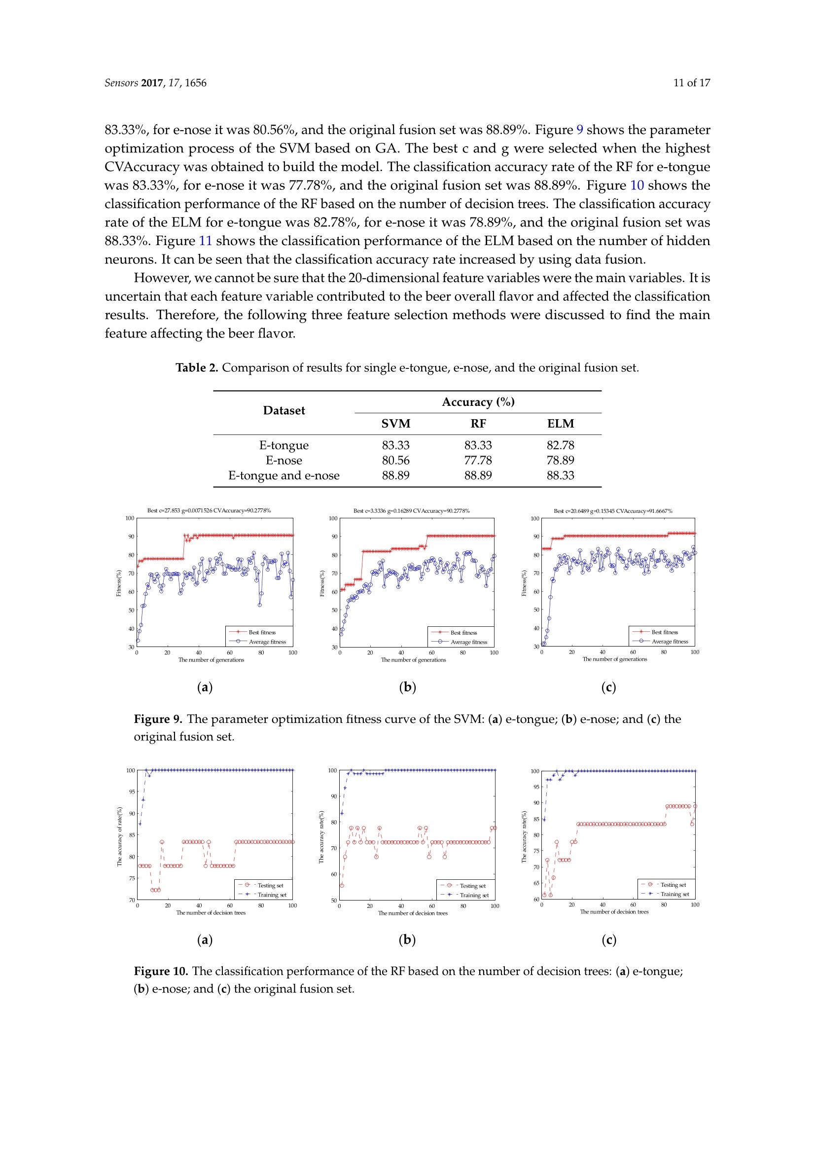
文章采用电子舌和电子鼻技术分析啤酒风味信息分类中的数据融合特征。首先,电子舌和电子鼻被用来收集味道和啤酒的嗅觉信息。第二,主成分分析(PCA),遗传算法-偏 小二乘(GA-PLS)和可变重要性的投影(VIP)评分将该方法应用于原始融合集特征变量的选择在SVM、RF和ELM上为评价特征挖掘方法的有效性而建立。
方案详情

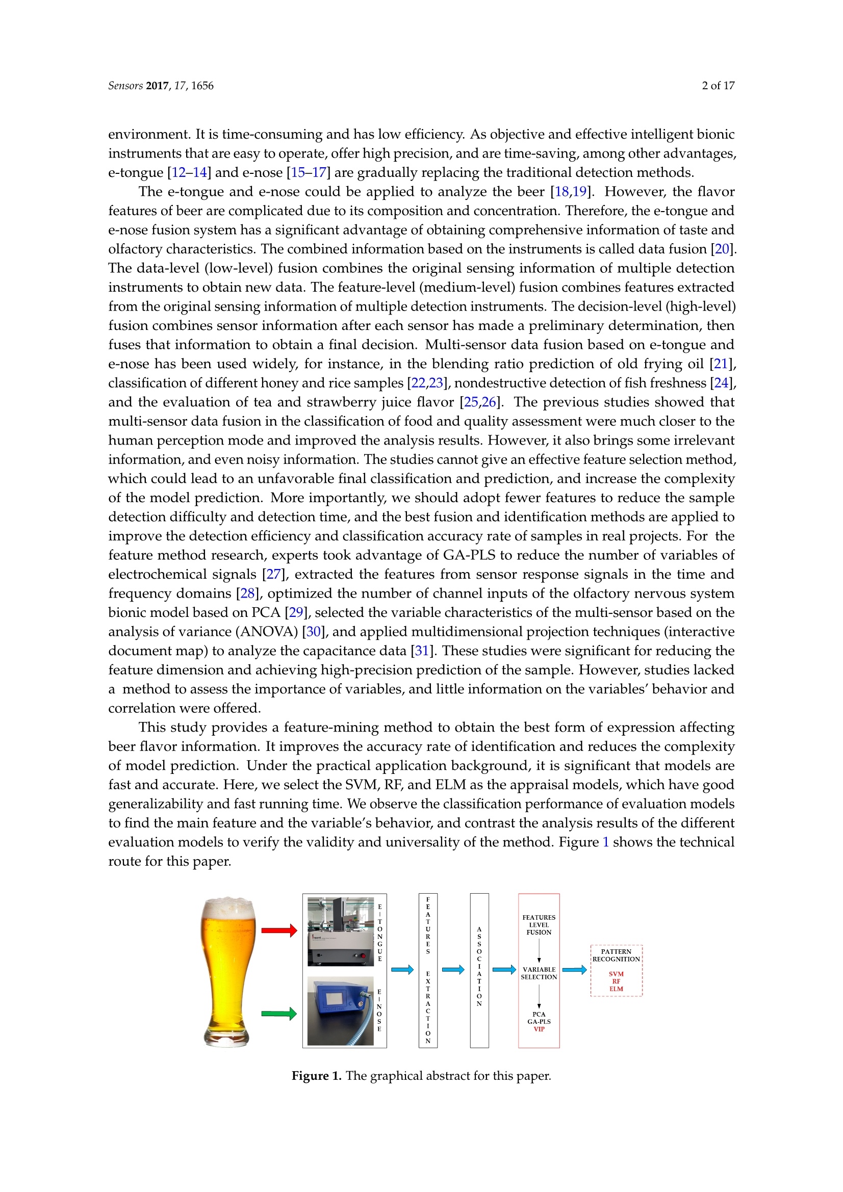
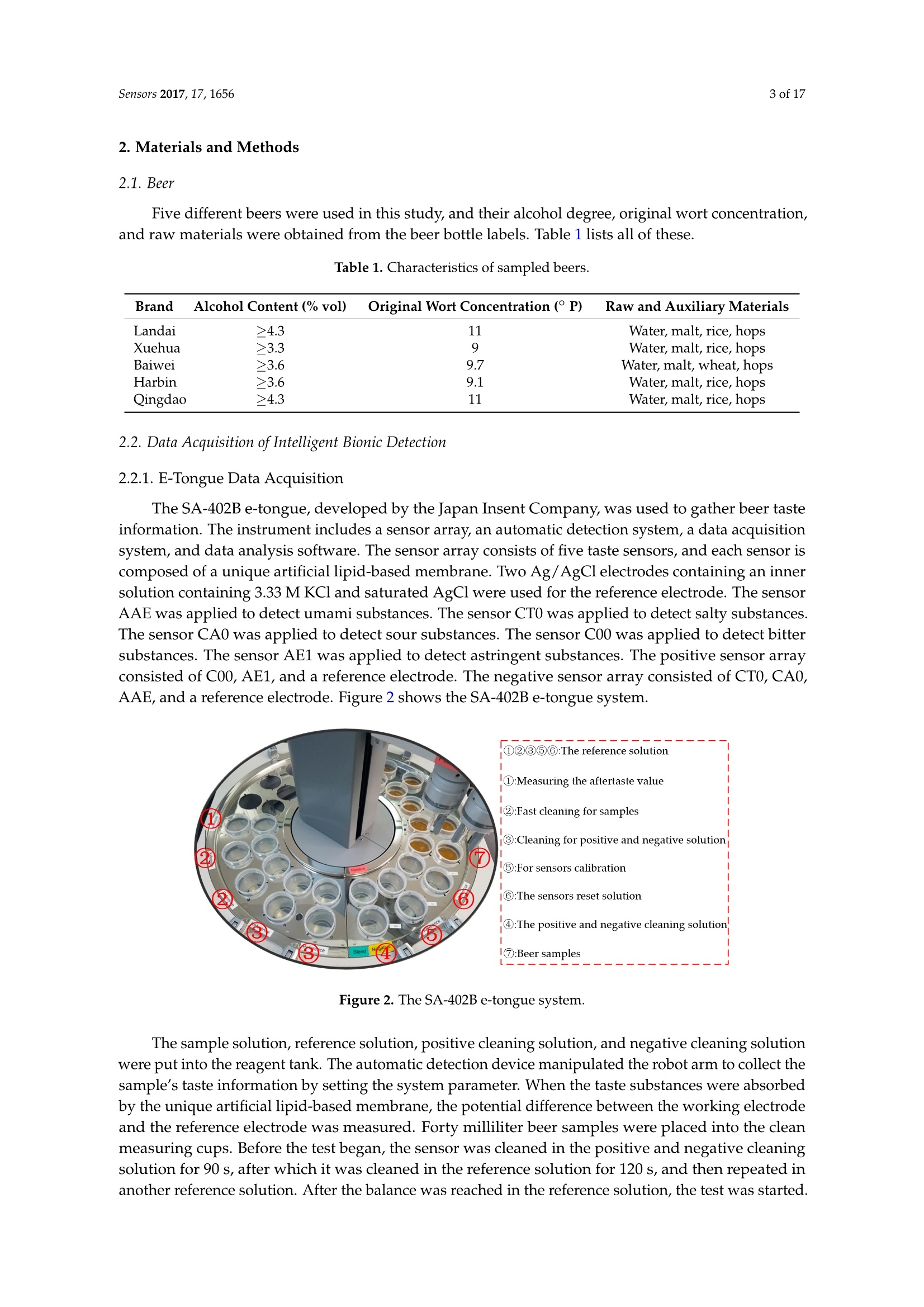
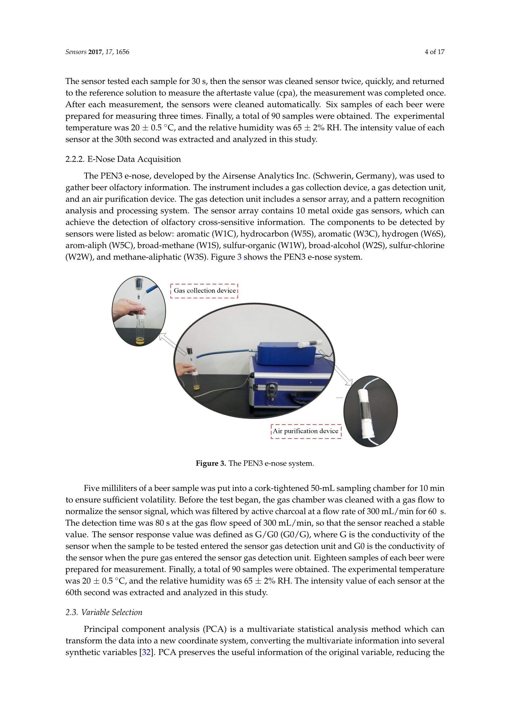
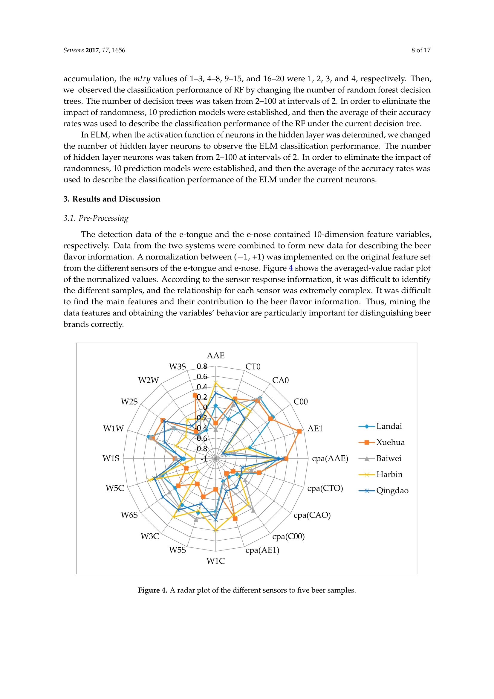
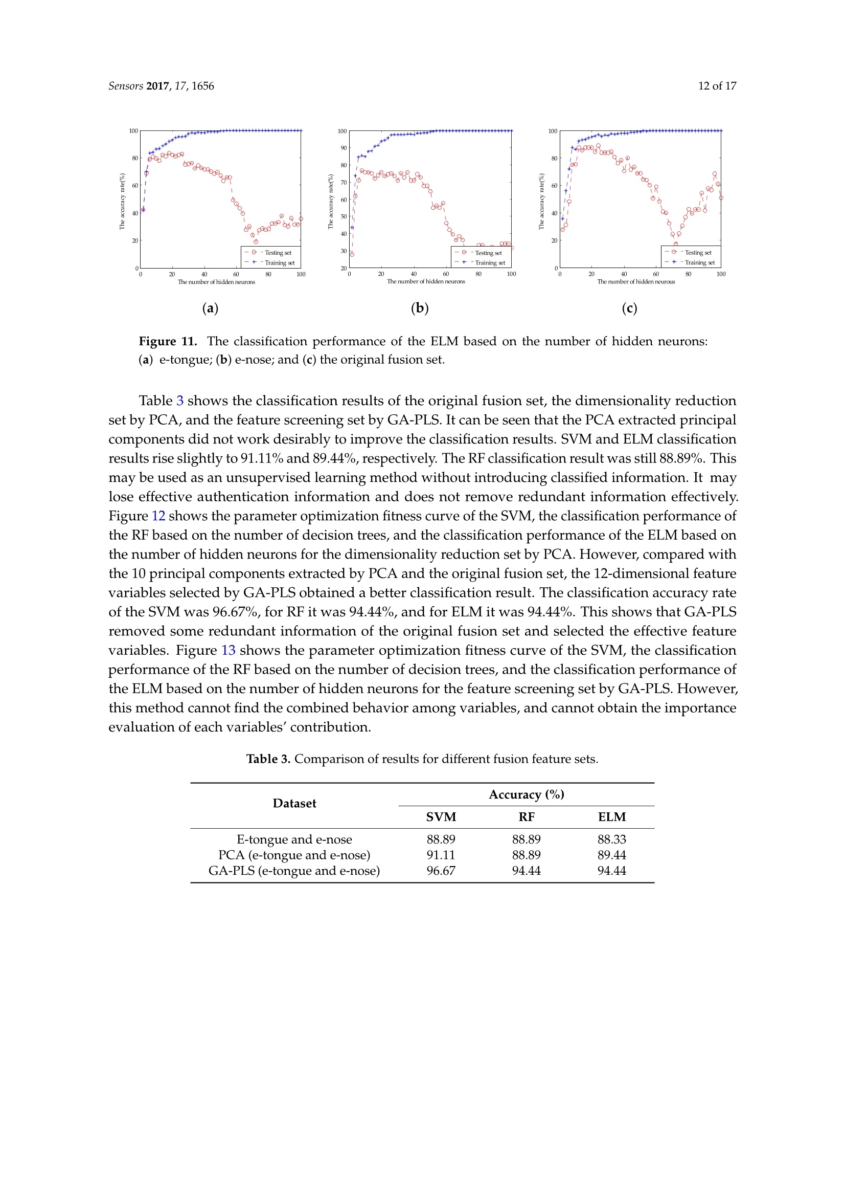
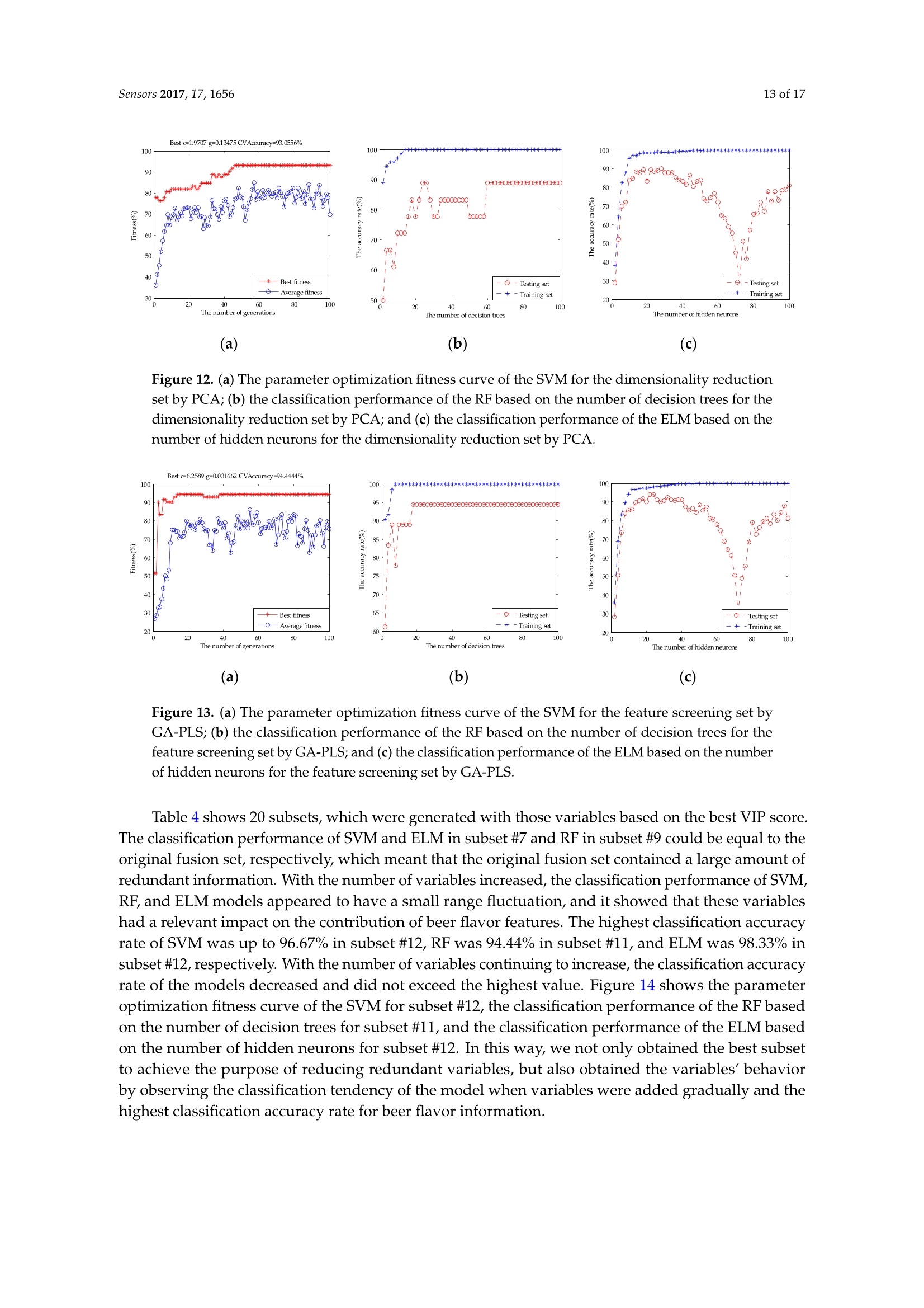
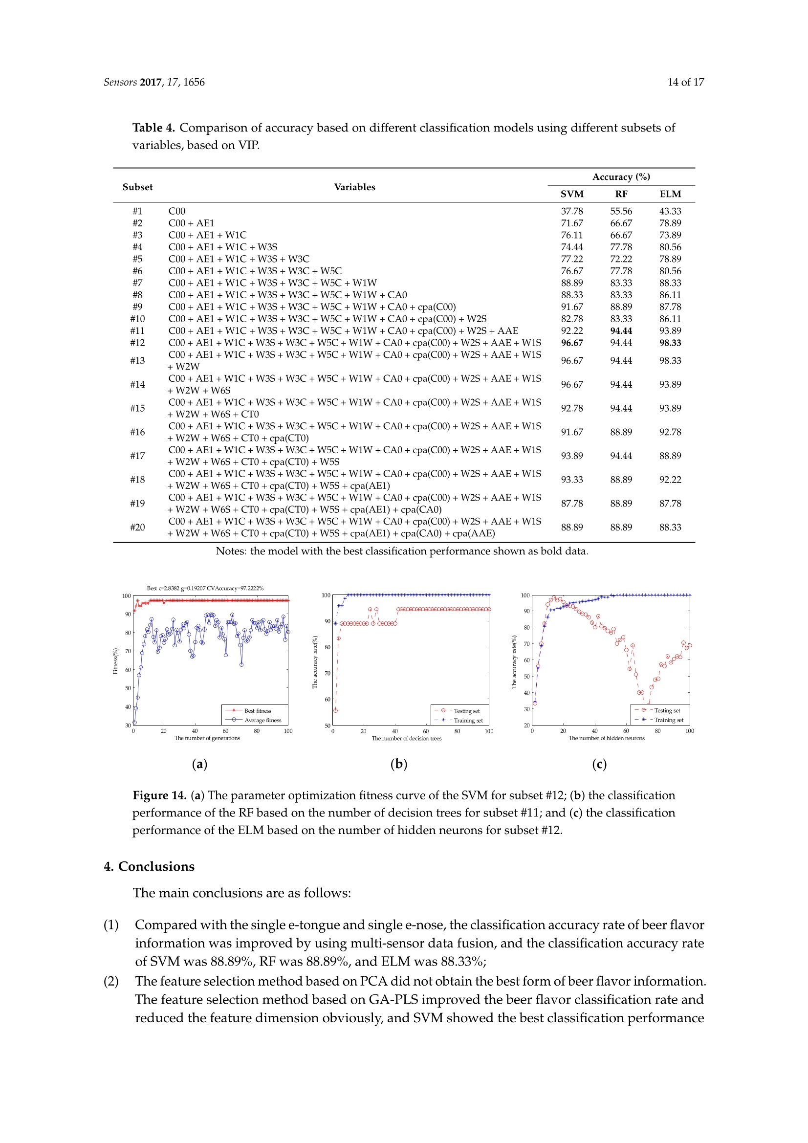
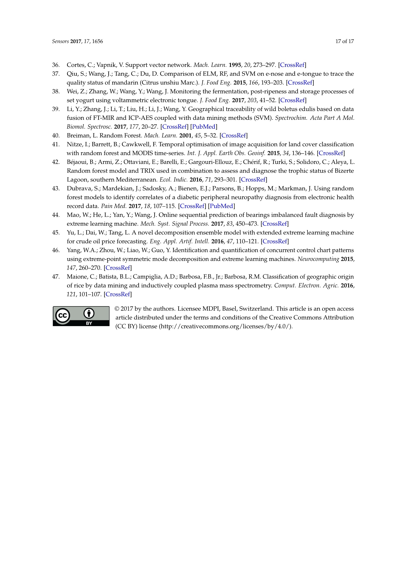
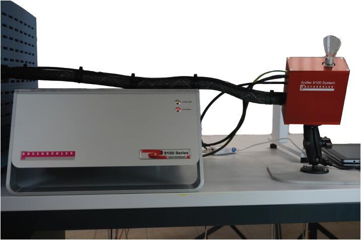
sensorS Sensors 2017, 17,16562 of 17 Sensors 2017,17,1656;doi:10.3390/s17071656www.mdpi.com/journal/sensors Article Mining Feature of Data Fusion in the Classification ofBeer Flavor Information Using E-Tongue and E-Nose Hong Men, Yan Shi, Songlin Fu, Yanan Jiao, Yu Qiao and Jingjing Liu * College of Automation Engineering, Northeast Electric Power University, Jilin 132012, China; menhong@neepu.edu.cn (H.M.); 2201500430@neepu.edu.cn (Y.S.); 2201500474@neepu.edu.cn (S.F.); 2201600437@neepu.edu.cn (Y.J.); 2201600453@neepu.edu.cn (Y.Q.) *Correspondence: jingjing _liu@neepu.edu.cn; Tel.:+86-432-6480-7283; Fax:+86-432-6480-6201 Received: 31 May 2017; Accepted: 14 July 2017; Published: 19 July 2017 Abstract: Multi-sensor data fusion can provide more comprehensive and more accurate analysisresults. However, it also brings some redundant information, which is an important issue with respectto finding a feature-mining method for intuitive and efficient analysis. This paper demonstratesa feature-mining method based on variable accumulation to find the best expression form andvariables' behavior affecting beer flavor. First, e-tongue and e-nose were used to gather the tasteand olfactory information of beer, respectively. Second, principal component analysis (PCA), geneticalgorithm-partial least squares (GA-PLS), and variable importance of projection (VIP) scores wereapplied to select feature variables of the original fusion set. Finally, the classification models basedon support vector machine (SVM), random forests (RF), and extreme learning machine (ELM) wereestablished to evaluate the efficiency of the feature-mining method. The result shows that thefeature-mining method based on variable accumulation obtains the main feature affecting beer flavorinformation, and the best classification performance for the SVM, RF, and ELM models with 96.67%,94.44%, and 98.33% prediction accuracy, respectively. Keywords: e-tongue; e-nose; data fusion; feature mining; variable accumulation; beer 1. Introduction The consumption of beer, as a beverage, ranks third in the world after water and tea. It is richin various amino acids, vitamins, and other nutrients needed by the human body [1,2], which iseuphemistically known as liquid bread’. Barley germination is the main raw material for beerbrewing, which makes beer a low-alcohol and high-nutrition drink. Additionally, it promotes digestion,spleen activity, appetite, and other functions [3-5]. Flavor information is one of the reference factors that reflects the beer’s features, which consistsof taste and olfactory information. Due to different manufacturing processes, both the taste andthe smell of different beers are different. According to consumer preference, they choose beers withdifferent flavors. Therefore, accurately and efficiently identifying different beers, and finding importantfeatures, are particularly significant. Meanwhile, it is also meaningful for quality control, storage,and authenticity recognition. A crucial observation was obtained in the psychology literature thatthe intensity of the senses could be overlapped, and people usually mistake volatile substances as'taste'[6]. When we cannot smell, it is difficult to distinguish apple and potato, red wine and coffee.The food odor can stimulate people to salivate, which improves our sensation. When drinking fruitjuice with the nose squeezed, sweet and sour can be felt by the tongue. Setting the nose free afterdrinking, the fruit juice flavor information will appear, so the sensory experience of food must be fullydependent on both the tongue and nose [7]. The conventional physical and chemical analysis methodscannot reflect the flavor characteristics of beer [8-10]. The most used method is sensory evaluation [11],but this method is quite subjective since the evaluation result changes with the physical condition and environment. It is time-consuming and has low efficiency. As objective and effective intelligent bionicinstruments that are easy to operate, offer high precision, and are time-saving, among other advantages,e-tongue [12-14] and e-nose [15-17] are gradually replacing the traditional detection methods. The e-tongue and e-nose could be applied to analyze the beer [18,19]. However, the flavorfeatures of beer are complicated due to its composition and concentration. Therefore, the e-tongue ande-nose fusion system has a significant advantage of obtaining comprehensive information of taste andolfactory characteristics. The combined information based on the instruments is called data fusion [20].The data-level (low-level) fusion combines the original sensing information of multiple detectioninstruments to obtain new data. The feature-level (medium-level) fusion combines features extractedfrom the original sensing information of multiple detection instruments. The decision-level (high-level)fusion combines sensor information after each sensor has made a preliminary determination, thenfuses that information to obtain a final decision. Multi-sensor data fusion based on e-tongue ande-nose has been used widely, for instance, in the blending ratio prediction of old frying oil [21],classification of different honey and rice samples [22,23], nondestructive detection of fish freshness [24],and the evaluation of tea and strawberry juice flavor [25,26]. The previous studies showed thatmulti-sensor data fusion in the classification of food and quality assessment were much closer to thehuman perception mode and improved the analysis results. However, it also brings some irrelevantinformation, and even noisy information. The studies cannot give an effective feature selection method,which could lead to an unfavorable final classification and prediction, and increase the complexityof the model prediction. More importantly, we should adopt fewer features to reduce the sampledetection difficulty and detection time, and the best fusion and identification methods are applied toimprove the detection efficiency and classification accuracy rate of samples in real projects. For thefeature method research, experts took advantage of GA-PLS to reduce the number of variables ofelectrochemical signals [27], extracted the features from sensor response signals in the time andfrequency domains [28], optimized the number of channel inputs of the olfactory nervous systembionic model based on PCA [29], selected the variable characteristics of the multi-sensor based on theanalysis of variance (ANOVA) [30], and applied multidimensional projection techniques (interactivedocument map) to analyze the capacitance data [31]. These studies were significant for reducing thefeature dimension and achieving high-precision prediction of the sample. However, studies lackeda method to assess the importance of variables, and little information on the variables' behavior andcorrelation were offered. This study provides a feature-mining method to obtain the best form of expression affectingbeer flavor information. It improves the accuracy rate of identification and reduces the complexityof model prediction. Under the practical application background, it is significant that models arefast and accurate. Here, we select the SVM, RF, and ELM as the appraisal models, which have goodgeneralizability and fast running time. We observe the classification performance of evaluation modelsto find the main feature and the variable's behavior, and contrast the analysis results of the differentevaluation models to verify the validity and universality of the method. Figure 1 shows the technicalroute for this paper. Figure 1. The graphical abstract for this paper. 2. Materials and Methods 2.1. Beer Five different beers were used in this study, and their alcohol degree, original wort concentration,and raw materials were obtained from the beer bottle labels. Table 1 lists all of these. Table 1. Characteristics of sampled beers. Brand Alcohol Content (% vol) Original Wort Concentration(°P) Raw and Auxiliary Materials Landai ≥4.3 11 Water, malt, rice, hops Xuehua ≥3.3 9 Water, malt, rice, hops Baiwei ≥3.6 9.7 Water, malt, wheat, hops Harbin ≥3.6 9.1 Water, malt, rice, hops Qingdao ≥4.3 11 Water, malt, rice, hops 2.2. Data Acquisition of Intelligent Bionic Detection 2.2.1. E-Tongue Data Acquisition The SA-402B e-tongue, developed by the Japan Insent Company, was used to gather beer tasteinformation. The instrument includes a sensor array, an automatic detection system, a data acquisitionsystem, and data analysis software. The sensor array consists of five taste sensors, and each sensor iscomposed of a unique artificial lipid-based membrane. Two Ag/AgCl electrodes containing an innersolution containing 3.33 M KCl .551and saturated AgCl were used for the reference electrode. The sensorAAE was applied to detect umami substances. The sensor CT0 was applied to detect salty substances.The sensor CA0 was applied to detect sour substances. The sensor C00 was applied to detect bittersubstances. The sensor AE1 was applied to detect astringent substances. The positive sensor arrayconsisted of C00, AE1, and a reference electrode. The negative sensor array consisted of CT0, CA0,AAE, and a reference electrode. Figure 2 shows the SA-402B e-tongue system. Figure 2. The SA-402B e-tongue system. The sample solution, reference solution, positive cleaning solution, and negative cleaning solutionwere put into the reagent tank. The automatic detection device manipulated the robot arm to collect thesample's taste information by setting the system parameter. When the taste substances were absorbedby the unique artificial lipid-based membrane, the potential difference between the working electrodeand the reference electrode was measured. Forty milliliter beer samples were placed into the cleanmeasuring cups. Before the test began, the sensor was cleaned in the positive and negative cleaningsolution for 90 s, after which it was cleaned in the reference solution for 120 s, and then repeated inanother reference solution. After the balance was reached in the reference solution, the test was started. The sensor tested each sample for 30 s, then the sensor was cleaned sensor twice, quickly, and returnedto the reference solution to measure the aftertaste value (cpa), the measurement was completed once.After each measurement, the sensors were cleaned automatically. Six samples of each beer wereprepared for measuring three times. Finally, a total of 90 samples were obtained. The experimentaltemperature was 20 ±0.5°C, and the relative humidity was 65 ±2% RH. The intensity value of eachsensor at the 30th second was extracted and analyzed in this study. 2.2.2. E-Nose Data Acquisition The PEN3 e-nose, developed by the Airsense Analytics Inc. (Schwerin, Germany), was used togather beer olfactory information. The instrument includes a gas collection device, a gas detection unit,and an air purification device. The gas detection unit includes a sensor array, and a pattern recognitionanalysis and processing system. The sensor array contains 10 metal oxide gas sensors, which canachieve the detection of olfactory cross-sensitive information. The components to be detected bysensors were listed as below: aromatic (W1C), hydrocarbon (W5S), aromatic (W3C), hydrogen (W6S),arom-aliph (W5C), broad-methane (W1S), sulfur-organic (W1W), broad-alcohol (W2S), sulfur-chlorine(W2W), and methane-aliphatic (W3S). Figure 3 shows the PEN3 e-nose system. Figure 3. The PEN3 e-nose system. Five milliliters of a beer sample was put into a cork-tightened 50-mL sampling chamber for 10 minto ensure sufficient volatility. Before the test began, the gas chamber was cleaned with a gas flow tonormalize the sensor signal, which was filtered by active charcoal at a flow rate of 300 mL/min for 60 s.The detection time was 80 s at the gas flow speed of 300 mL/min,so that the sensor reached a stablevalue. The sensor response value was defined as G/G0 (G0/G),where G is the conductivity of thesensor when the sample to be tested entered the sensor gas detection unit and G0 is the conductivity ofthe sensor when the pure gas entered the sensor gas detection unit. Eighteen samples of each beer wereprepared for measurement. Finally, a total of 90 samples were obtained. The experimental temperaturewas 20 ±0.5°C, and the relative humidity was 65 ±2% RH. The intensity value of each sensor at the60th second was extracted and analyzed in this study. 2.3. Variable Selection Principal component analysis (PCA) is a multivariate statistical analysis method which cantransform the data into a new coordinate system, converting the multivariate information into severalsynthetic variables [32]. PCA preserves the useful information of the original variable, reducing the dimension of the multidimensional dataset,and extracts the principal component. The number ofprincipal components is calculated according to the maximum variance principle. We determinedthe number of principal components according to the cumulative contribution rate and practicalrequirements. In this work, in order to obtain as much information as possible from the original fusionset, we made sure that the principal component with a cumulative variance contribution was 99%. The feature variables can be screened by genetic algorithm-partial least squares (GA-PLS) toremove redundant variables for constructing the classification model [33,34]. In the process ofvariable selection, a randomization test is used to determine whether it can be applied; usually,the randomization test value is less than 5. As the number of variables increases, the cross-validatedexceptions variance (CV%) value gradually increases to reach a maximum, and finally maintainsa relatively stable state. Meanwhile, the root mean square error of cross-validation (RMSECV)gradually decreases to reach a minimum, and finally maintains a relatively stable state. In thecalculation process, the chromosome corresponds to the highest CV%, and smallest RMSECV is thebest optimal variable subset. In the PLS, the explanatory ability of the independent variable to the dependent variable ismeasured by the variable importance of projection (VIP) scores [35]. The marginal contribution of theindependent variable to the principal component is called VIP. The VIP definition is based on the factthat the explanatory ability of the independent variable to the dependent variable is passed through t,and if the explanatory ability of t to the dependent variable is strong, and the independent variableplays a very important role for t, we think that the explanatory ability of the independent variable tothe dependent variable will be large. In this study, the variable importance of the e-tongue and e-nosefusion set is sorted based on the VIP scores. 2.4. Multivariate Analysis 2.4.1. Support Vector Machines (SVM) SVM was first proposed by Cortes and Vapnik [36], and is a supervised learning model forclassification and regression. The main idea is to establish a classification hyperplane as a decisionplane. The SVM uses the kernel function to map the data to the high-dimensional space, making it aslinear as possible. The kernel functions include linear kernel, polynomial kernel, radial basis kernel(RBF), Fourier kernel, spine kernel, and sigmoid nucleus in SVM. Compared with the kernel functionand previous studies, the RBF kernel function gave an excellent classification performance [37-39].Whether the sample is small or large, high dimension or low dimension, the RBF kernel function isapplicable. Therefore, this paper used the RBF as the SVM classification kernel function. The SVM algorithm proceeds as follows: Set the detected data vector to be N-dimensional, and then the L sets can be represented as(x1,y1)….,(xi,yi) E R". The hyperplane constructed as: where ω is the weight coefficient of the decision plane, p(x) is a nonlinear mapping function, and bis the domain value for the category division. In order to minimize the structural risk, the optimalclassification plane satisfies the condition as: Introducing the nonnegative slack variable Gi, the classification error is allowed within a certainrange. Therefore, the optimization problem is translated into: where c is the penalty factor to control the complexity and approximation error of the model,and determine the generalizability of the SVM. Here, introducing the Lagrange multiplier algorithm,the optimization problem is transformed into dual form: 1=1 where: In this paper, the RBF kernel function is introduced: where g is the kernel function parameter, which is related to the input space range or width. The largerthe sample input space range is, the larger the value is. In contrast, the smaller the sample input spacerange is, the smaller the value is. The above optimization problem is translated into: Therefore, the minimization problem depends on the parameters c and g, and the correct andeffective selection of parameters would show a good classification performance for SVM. Thus,GA was combined with SVM to optimize the penalty factor c and the kernel function parameter g.The parameters of the GA are initialized as follows: maximum generation was 100, population was 20,the search range of c was 0 to 100, and that of g was 0 to 1000. 2.4.2. Random Forests (RF) RF is a nonlinear classification and regression algorithm, which was first proposed by Tin Kam in1995. In 2001, Breiman conducted a deeper research [40]. The method combines bootstrap aggregatingand random subspace successfully.. The essence of RF is a classifier that contains a number ofdecision trees that are not associated with each other. When the data is input into a random forest,the classification result is recorded by each decision tree. Finally, the category of data is voted bydecision trees. The RF shows good efficiency in practical applications, such as image processing,environmental monitoring, and medical diagnosis [41-43]. The RF algorithm proceeds as follows: ①Using bootstrap sampling to generate T training sets S1,S2.…·,Sr randomly; Each training set is used to generate the decision tree C1,C2…,Cr. The value of the splitproperty set for each tree is mtry. The mtry value is the square root of the number of inputvariables. In general, the value of mtry remains stable throughout the forest development process; Each tree has a complete development without taking pruning; For testing setX, each decision treeeislsuusedtotestand obtain the:0categoryC1(X),C2(X),…·,Cr(X); and (5) The category of the testing set is voted by decision trees. 2.4.3. Extreme Learning Machine (ELM) Extreme learning machine (ELM) is a new algorithm for regression and classification, which wasfirst proposed by Huang of Nanyang Technological University [40]. The essence of ELM is a single hidden layer feed-forward neural network (SLFN). The difference with other SLFN is that ELMrandomly generates the connection weights (w) and threshold (b), and without adjustment in thetraining process. The optimal results can be obtained by adjusting the number of neurons in the hiddenlayer. Compared with the traditional training methods, this method has the advantages of fast learningspeed and good generalization performance. In recent years, ELM has gained attention widely, such aswith on-line fault monitoring, price forecasting, and control chart pattern recognition [44-46]. N samples are described by (xi,t;), where xi=[xx1xx2…,xxn]eR",t;=[ti,xi2;,tim]e R".The activation function of neurons in the hidden layer is G. The ELM model can be represented as: where a; =[1,a2,an] is the weight vector of the ith hidden layer node and the input node.pi=[B1,B2…,Bn] is the weight vector of the ith hidden layer node and the input node. b; is thethreshold of the ith hidden node.N is the number of hidden neurons. Equation (8) can beabbreviated as: where: where H is the output matrix of the hidden layer, and the output weights can be obtained by solvingthe least squares solution of the linear equations: The least squares solution as: where H+is the Moore-Penrose generalized inverse of the hidden layer output matrix H. 2.5. Allocation ofDatasets and the Model Prediction Process The 90 samples of original data were divided into two groups randomly. One group included72 samples, which was used as a training set to build the model. The remaining 18 samples were usedas a testing set to verify the classification performance of the model. In SVM, in order to avoid over-learning and insufficient learning when searching the bestparameters, the fitness function value of the GA was the highest accuracy rate of the training setunder five-fold cross-validation, and the best c and g were selected when the highest CVAccuracywas obtained. In order to eliminate the impact of randomness,10 prediction models were established,and then the average of their accuracy rates was used to describe the classification performance ofthe SVM. In RF, the mtry value is the square root of the number of input variables. Therefore, the mtry valueof single e-tongue, single e-nose, the dimensionality reduction set by PCA, and the feature screeningset by GA-PLS were 3. The mtry value of original fusion set was 4. The 20 subsets based on variable accumulation, the mtry values of 1-3, 4-8, 9-15, and 16-20 were 1, 2,3, and 4, respectively. Then,we observed the classification performance of RF by changing the number of random forest decisiontrees. The number of decision trees was taken from 2-100 at intervals of 2. In order to eliminate theimpact of reandomness, 10 prediction models were established, and then the average of their accuracyrates was used to describe the classification performance of the RF under the current decision tree. In ELM, when the activation function of neurons in the hidden layer was determined, we changedthe number of hidden layer neurons to observe the ELM classification performance. The numberof hidden layer neurons was taken from 2-100 at intervals of 2. In order to eliminate the impact ofrandomness, 10 prediction models were established, and then the average of the accuracy rates wasused to describe the classification performance of the ELM under the current neurons. 3. Results and Discussion 3.1. Pre-Processing The detection data of the e-tongue and the e-nose contained 10-dimension feature variables,respectively. Data from the two systems were combined to form new data for describing the beerflavor information. A normalization between (-1, +1) was implemented on the original feature setfrom the different sensors of the e-tongue and e-nose. Figure 4 shows the averaged-value radar plotof the normalized values. According to the sensor response information, it was difficult to identifythe different samples, and the relationship for each sensor was extremely complex. It was difficultto find the main features and their contribution to the beer flavor information. Thus, mining thedata features and obtaining the variables' behavior are particularly important for distinguishing beerbrands correctly. Figure 4. A radar plot of the different sensors to five beer samples. 3.2. Extraction of Sensor Feature Variables In order to acquire as much information as possible from the original fusion set, the 10 principalcomponents were extracted by PCA, and the accumulated variance contribution rate was as highas 99.99%. Before applying the GA-PLS to select variables, a randomization test was required to determinewhether it could be applied. Figure 5 shows that randomization test result of the original fusion set.It can be seen that the randomization test value was less than 5, indicating that the GA-PLS wasreliable. Figure 6 shows the GA-PLS search process for the best number of variables, it can be seenthat the CV% increased rapidly and then gradually slowed down as the number of variables increases.When CV% reached a maximum 82.169%, the number of variables reached 12, and the number ofvariables continued to increase, the CV% decreased slightly and then stayed in a relatively stable state.On the contrary, in Figure 7, RMSECV decreased rapidly, and then slowly with the increase in thenumber of variables. When the number of variables reached 12, the RMSECV arrived at its minimumvalue of 0.5937, and then as the number of variables continued to increase, RMSECV increased slightlyand maintained a relatively stable state. Finally, 12 feature variables were extracted from the originalfusion set, which were CA0, C00, AE1, AAE, cpa(C00), W1C, W5S, W6S, W1S, W1W, W2S, and W2W. Figure 5. Randomization test result. 00丫 0 Figure 6. CV% change curve. Figure 7. RMSECV change curve. Figure 8 shows the VIP score of the original variables of the e-tongue and e-nose. C00 and AE1 hadlarger VIP scores than the other variables, and this means that bitter and astringent were significant forbeer classification.Cpa(AAE) and cpa(CA0) had smaller VIP scores, and this means that the aftertasteof umami and sour were less important for beer flavor. Thus, we generated the variable subsets whichcould be used to build the classification models. Each subset was generated with those variablesbased on the best VIP score. Subset #1 included C00, subset #2 included C00 and AE1, and subset #20contained all the variables of the e-tongue and the e-nose. We then gradually accumulated the numberof variables, and observed the classification results of the models to achieve the purpose of filteringredundant information [47]. Figure 8. Ranking the importance of variables based on the VIP score. 3.3. Results of the Models Table 2 shows the classification results of single e-tongue, single e-nose, and the original fusionset based on the SVM, RF, and ELM. The classification accuracy rate of the SVM for e-tongue was 83.33%, for e-nose it was 80.56%, and the original fusion set was 88.89%. Figure 9 shows the parameteroptimization process of the SVM based on GA. The best c and g were selected when the highestCVAccuracy was obtained to build the model. The classification accuracy rate of the RF for e-tonguewas 83.33%, for e-nose it was 77.78%, and the original fusion set was 88.89%. Figure 10 shows theclassification performance of the RF based on the number of decision trees. The classification accuracyrate of the ELM for e-tongue was 82.78%, for e-nose it was 78.89%, and the original fusion set was88.33%. Figure 11 shows the classification performance of the ELM based on the number of hiddenneurons. It can be seen that the classification accuracy rate increased by using data fusion. However,we cannot be sure that the 20-dimensional feature variables were the main variables. It isuncertain that each feature variable contributed to the beer overall flavor and affected the classificationresults. Therefore, the following three feature selection methods were discussed to find the mainfeature affecting the beer flavor. Table 2. Comparison of results for single e-tongue, e-nose, and the original fusion set. (a) (b) (C) Figure 9. The parameter optimization fitness curve of the SVM: (a)e-tongue; (b) e-nose; and (c) theoriginal fusion set. (a) (b) (c) Figure 10. The classification performance of the RF based on the number of decision trees: (a) e-tongue;(b) e-nose;and (c) the original fusion set. Figure 11. The classification performance of the ELM based on the number of hidden neurons:(a) e-tongue; (b) e-nose; and (c) the original fusion set. Table 3 shows the classification results of the original fusion set, the dimensionality reductionset by PCA, and the feature screening set by GA-PLS. It can be seen that the PCA extracted principalcomponents did not work desirably to improve the classification results. SVM and ELM classificationresults rise slightly to 91.11% and 89.44%, respectively. The RF classification result was still 88.89%. Thismay be used as an unsupervised learning method without introducing classified information. It maylose effective authentication information and does not remove redundant information effectively.Figure 12 shows the parameter optimization fitness curve of the SVM, the classification performance ofthe RF based on the number of decision trees, and the classification performance of the ELM based onthe number of hidden neurons for the dimensionality reduction set by PCA. However, compared withthe 10 principal components extracted by PCA and the original fusion set, the 12-dimensional featurevariables selected by GA-PLS obtained a better classification result. The classification accuracy rateof the SVM was 96.67%, for RF it was 94.44%, and for ELM it was 94.44%. This shows that GA-PLSremoved some redundant information of the original fusion set and selected the effective featurevariables. Figure 13 shows the parameter optimization fitness curve of the SVM, the classificationperformance of the RF based on the number of decision trees, and the classification performance ofthe ELM based on the number of hidden neurons for the feature screening set by GA-PLS. However,this method cannot find the combined behavior among variables, and cannot obtain the importanceevaluation of each variables'contribution. Table 3. Comparison of results for different fusion feature sets. Dataset Accuracy(%) SVM RF ELM E-tongue and e-nose 88.89 88.89 88.33 PCA (e-tongue and e-nose) 91.11 88.89 89.44 GA-PLS (e-tongue and e-nose) 96.67 94.44 94.44 (a) (b) (c) Figure 12. (a) The parameter optimization fitness curve of the SVM for the dimensionality reductionset by PCA; (b) the classification performance of the RF based on the number of decision trees for thedimensionality reduction set by PCA; and(c) the classification performance of the ELM based on thenumber of hidden neurons for the dimensionality reduction set by PCA. (a) (b) (c) Figure 13. (a) The parameter optimization fitness curve of the SVM for the feature screening set byGA-PLS; (b) the classification performance of the RF based on the number of decision trees for thefeature screening set by GA-PLS; and (c) the classification performance of the ELM based on the numberof hidden neurons for the feature screening set by GA-PLS. Table 4 shows 20 subsets, which were generated with those variables based on the best VIP score.The classification performance of SVM and ELM in subset #7 and RF in subset #9 could be equal to theoriginal fusion set, respectively, which meant that the original fusion set contained a large amount ofredundant information. With the number of variables increased, the classification performance of SVM,RF, and ELM models appeared to have a small range fluctuation, and it showed that these variableshad a relevant impact on the contribution of beer flavor features. The highest classification accuracyrate of SVM was up to 96.67% in subset #12, RF was 94.44% in subset #11, and ELM was 98.33% insubset #12, respectively. With the number of variables continuing to increase, the classification accuracyrate of the models decreased and did not exceed the highest value. Figure 14 shows the parameteroptimization fitness curve of the SVM for subset #12, the classification performance of the RF basedon the number of decision trees for subset #11, and the classification performance of the ELM basedon the number of hidden neurons for subset #12. In this way, we not only obtained the best subsetto achieve the purpose of reducing redundant variables, but also obtained the variables’ behaviorby observing the classification tendency of the model when variables were added gradually and thehighest classification accuracy rate for beer flavor information. Table 4. Comparison of accuracy based on different classification models using different subsets ofvariables, based on VIP. Subset Variables Accuracy (%) SVM RF ELM #1 C00 37.78 55.56 43.33 #2 C00 +AE1 71.67 66.67 78.89 #3 C00+AE1+W1C 76.11 66.67 73.89 #4 C00+AE1+W1C+W3S 74.44 77.78 80.56 #5 C00+AE1+W1C+W3S+ W3C 77.22 72.22 78.89 #6 C00+AE1+W1C+W3S+W3C+W5C 76.67 77.78 80.56 #7 C00+AE1+W1C+W3S+W3C+W5C+ W1W 88.89 83.33 88.33 #8 C00+AE1+W1C+W3S+W3C+W5C+W1W+CA0 88.33 83.33 86.11 #9 C00+AE1+W1C+ W3S+W3C+W5C+W1W+CA0+cpa(C00) 91.67 88.89 87.78 #10 C00+AE1+W1C +W3S+W3C+W5C+W1W+CA0+cpa(C00)+W2S 82.78 83.33 86.11 #11 C00+AE1+W1C+W3S+W3C+W5C+W1W+CA0+cpa(C00)+W2S+AAE 92.22 94.44 93.89 #12 C00+AE1+ W1C+ W3S+W3C+W5C+W1W+CA0+cpa(C00)+W2S+AAE+ W1S 96.67 94.44 98.33 #13 C00+AE1+W1C+ W3S+W3C+W5C+W1W+CA0+cpa(C00)+W2S+AAE+ W1S + W2W 96.67 94.44 98.33 #14 C00+AE1+W1C+W3S+W3C+W5C+W1W+CA0+cpa(C00)+W2S+AAE + W1S +W2W+W6S 96.67 94.44 93.89 #15 C00+AE1+ W1C + W3S+W3C+W5C+W1W+CA0+cpa(C00)+W2S+AAE+ W1S +W2W+W6S+CTO 92.78 94.44 93.89 #16 C00+AE1+W1C+W3S+W3C+W5C+W1W+CA0+cpa(C00)+W2S+AAE+ W1S +W2W+ W6S+ CT0 +cpa(CT0) 91.67 88.89 92.78 #17 C00+AE1 +W1C+W3S+W3C+W5C+W1W+CA0+cpa(C00)+W2S+AAE+W1S +W2W+W6S+CT0+cpa(CT0)+W5S 93.89 94.44 88.89 #18 C00+AE1+W1C+W3S+W3C+W5C+W1W+CA0+cpa(C00)+W2S+AAE+W1S +W2W+W6S+CT0+cpa(CT0)+ W5S+cpa(AE1) 93.33 88.89 92.22 #19 C00+AE1+ W1C+ W3S +W3C+W5C+W1W+CA0+ cpa(C00)+W2S+AAE + W1S + W2W +W6S+CT0+cpa(CT0)+ W5S + cpa(AE1)+cpa(CA0) 87.78 88.89 87.78 #20 C00+AE1+W1C+ W3S+W3C+W5C+W1W+CA0+cpa(C00)+W2S+AAE+ W1S +W2W+W6S+CT0+cpa(CT0)+ W5S +cpa(AE1)+cpa(CA0)+cpa(AAE) 88.89 88.89 88.33 Notes: the model with the best classification performance shown as bold data. 100 ***** 90 80 70 60 50 40 -Training set (a) (b) (c) Figure 14. (a) The parameter optimization fitness curve of the SVM for subset #12; (b) the classificationperformance of the RF based on the number of decision trees for subset #11; and (c) the classificationperformance of the ELM based on the number of hidden neurons for subset #12. 4. Conclusions The main conclusions are as follows: (1) Compared with the single e-tongue and single e-nose, the classification accuracy rate of beer flavorinformation was improved by using multi-sensor data fusion, and the classification accuracy rateof SVM was 88.89%, RF was 88.89%, and ELM was 88.33%; (2) The feature selection method based on PCA did not obtain the best form of beer flavor information.The feature selection method based on GA-PLS improved the beer flavor classification rate andreduced the feature dimension obviously, and SVM showed the best classification performance at 96.67%. However, it did not give the contribution behavior of each variable for the overallinformation; and (3) By variable accumulation based on the best VIP score, the classification accuracy rate of SVM andELM in subset #7 was 88.89% and 88.33%, respectively, and the classification accuracy rate of theRF in subset #9 was 88.89%, which meant that the original fusion set contained a lot of redundantinformation. Finally, ELM showed the best classification performance 98.33% in subset #12. Thus,C00, AE1, W1C,W3S, W3C, W5C, W1W,CA0, cpa(C00), W2S, AAE, and W1S were considered asthe main features. Among the contributions of this study, a variable accumulation strategy based on the best VIPscore was proposed and applied to beer flavor information identification. It provided a vital method,which used the least characteristic variables and the best fusion method,combined with excellentpattern recognition methods, to identify beer flavor information more efficiently and more accurately.It not only obtained the important evaluation of each variable, but also obtained the correlationbehavior by observing the classification tendency of the model. Meanwhile, it also provided a moreefficient and accurate method to monitor product quality in the actual process of industrialization. Acknowledgments: This work was supported by the National Natural Science Foundation of China(no. 31401569), the Key Science and Technology Project of Jilin Province (20170204004SF), the Scientific ResearchFoundation for Young Scientists of Jilin Province (20150520135JH), and the Graduate Innovation Fund Project ofNortheast Electric Power University (Y2016018). Author Contributions: Hong Men and Jingjing Liu conceived the experiment and analytical methods. Yan Shianalyzed the data and wrote the paper. Songlin Fu and Yanan Jiao performed the e-tongue and e-nose experimentto obtain the taste and olfactory information. Yu Qiao extracted the taste and olfactory characteristic information. Conflicts of Interest: The authors declare no conflict of interest. References ( 1. Denke, M.A. Nutritional and health benefits of beer . Am. J. Med. Sci. 2000, 320,320-326 . [ CrossRe f] [PubMed] ) ( 2. Lynch, K.M.; Steffen, E.J.; Arendt,E.K. Brewers’spent grain: A review w ith an emphasis on food and health.J. Inst. Brew. 2016,122,553-568. [Cros s Ref ) ( 3. Miranda, C.L.; Stevens, J.F.; Helmrich, A.; Henderson, M. C .; Rodriguez, R.J.; Yang, Y.H.; Dei n zer, M.L.;Barnes, D.W.; Buhler, D.R. Antiproliferative and cytotoxic effects of prenylated flavonoids from hops(Humulus lupulus) in h uman cancer cell lines. Food Chem. Toxic o l. 1999, 37, 271-285. [Cross Ref] ) ( 4. Pfeiffer , A.; Hogl , B.; Kaes s , H. Effect of ethanol and commonly ingested alcoholic beverages on gastricemptying and gastrointestinal t r ansit.J. Mol. Med. 1992,70, 487-491.[Cr ossRef] ) ( 5. Stevens, J.F.;Ivancic, M.; Hsu, V.L.; Deinzer, M.L. Prenylflavonoids from hu m ulus lupulus. Phytochemistry1997,44,1575-1585. [ CrossRef ) ( 6. Murphy, C.;Cain, W.S. Taste and olfaction: Ind e pendence vs interaction. Physiol. Behav . 1980, 24,601-605. [ C r ossRef l ) ( 7. Murphy, C.; Cain, W.S.; Bartoshuk, L.M. Mutual action of tas t e and olf a ction. Sens. Pr o cess. 1977,1,204-211. ) ( 8. Castro, L.F.; Ross, C.F. Determination of flavour compounds in beer using stir-bar sorptive extraction andsolid-phase microextraction. J. Inst. Brew. 2015,121,1 9 7-203. [Cr o s sRef] ) ( 9. Dong, J.J.; Li, Q.L.; Yin, H.;Zhong, C.;Hao,J.G.; Yang , P.F.; T ian, Y.H.; Jia,S.R. Predictive analysis of beerquality by correlating sensory evaluation with higher alcohol and ester production using multivariatestatistics methods. Food Chem. 2014, 161,376-382. [CrossRef ][ PubMed] ) ( 10. Ghasemi-Varnamkhasti, M.; Mohtasebi, S.S.;R o driguez-Mendez, M.L.;Lozano,J.; Raz a vi, S.H.; Ahmadi, H.;Apetrei, C. Classification of n on-alcoholic beer based on aftertaste sensory evaluation by chemometric tools.Expert Syst. Appl. 2012, 39,4315-4327.[C rossRef] ) ( 11. Bacci, L.; Camilli, F.; Drago, M.S.; Magli, M.; Vagnoni, E.; Mauro, A.; Predieri, S. Sensory evaluation andinstrumental measurements to determine tactile properties of wool fabrics. Tex t . Res. J. 2012,82,1430-1441. [ CrossRe f ) ( 12. Wang, L.; Niu, Q.; Hui, Y . ;Jin, H. Discrimination of ri c e with different pretreatment methods by using a voltammetric electronic tongue. Sensors 2015, 15, 17767-17785. [CrossRef ] [P ubMed] ) ( 13. Ciosek, P.; Wesoly, M.;Zabadaj, M. Towards flow-through/flow injection electronic tongue for the an a lysis of pharmaceuticals. Sens. Actuators B Chem . 2015,207,1087-1094. [ CrossRef ) ( 14. Cet6,X.; Gonzalez-Calabuig, A.; Crespo, N.; Pérez, S.; Capdevila, J.;Puig-Pujol, A.; Valle, M.D. Electronictongues to assess wine sensory descriptors. T alanta 2016,162,218-224. [ C r ossRef][P ub Med] ) ( 15. Romain, A.C.; Godefroid, D.; Kuske,M.;Nicolas, J. Monitoring the exhaust air of a compost pile as a process variable with an e-nose. Sens. Actuators B Chem. 2005, 106,29-35.[Cr ossRef] ) ( 16. Zhu, J.C.; Feng, C. ; Wang, L.Y.; Niu, Y.W.; Xiao,Z.B. Evaluation of the synergism among volatile compoundsin oolong tea infusion by odour threshold with sensory analysis and e-nose. Food Chem. 2017, 221, 1484-1490.[ CrossRef ] [PubMed] ) ( 17. Li, Q.;Gu, Y.; Jia, J. Classification of multiple chinese liquors by means ofa QCM-based e-nose and MDS-SVMclassifier. Sensors 2017, 17,272 .[CrossRe f] [PubMed ] ) ( 18. Ghasemi-Varnamkhasti, M.; Mohtasebi, S.S . ; Si a dat, M.; Lozano,J.; Ahmadi, H.; Razavi, S.H.; Dicko, A.Aging f i ngerprint characterization of beer using electronic nose. Sens. Actuators B Chem. 2011, 1 5 9, 51-59. [ C r ossRef l ) ( 19. Ceto, X .; Gutierrez-Capitán, M . ; Calvo, D. ; De l , V.M. Beer classification by means of a potentiometricelectronic tongue. Food Chem. 2013,141,2533-2540. [CrossRe f ] [PubMed ] ) ( 20. Banerjee, R.; Tudu, B.; Bandyopadhyay, R.;Bhattacharyya, N. A review on combined odor and taste s e nsorsystems. J. Food Eng. 2016,190,10-21.[C rossRef] ) ( 21. Men, H.; Chen, D.; Z h ang, X.; Liu,J; Ning, K. D at a fusion of electronic nose and electronic tongue fordetection of mixed edible-oil. J . Sens. 2 014, 2014,1-7. [Cr o s sRef] ) ( 22. Zakaria, A.; Shakaff, A.Y.; Masnan, M .J.; Ahmad, M.N.; Adom, A.H. ; Jaaf a r, M.N.; Ghani, S.A.;Abdullah, A .H.; A ziz, A.H.; K amarudin, L.M. A biomimetic sensor for the classification of honeys ofdifferent floral origin an d the detection of adulteration. Sensors 2010, 11,7799-782 2 . [CrossRe f] [PubMed ] ) ( 23. Lu, L.; Deng, S.; Zhu, Z.; Tian, S . Classification of rice by combining electronic tongue and nose. Food Anal.Methods 2015,8, 1893-1902. [ C r ossRef] ) ( 24. Han, F; Huang, X.; Teye,E. ; Gu, F.; Gu, H. Nondestructive detection of fish freshness during its preservation by combining electronic nose and el e ctronic tongue techniques in conjunction with chemometric analysis. Anal. Methods 2014, 6,529-536. [ CrossRef] ) ( 25. Pan,J;Duan, Y;Jiang, Y.;Lv, Y.; Zhang, H.; Zhu, Y.; Zhang, S. Evaluation of fuding white tea flavor using electronic nose and electronic tongue. Sci. Technol . Food Ind. 2017,38,25-43. [CrossRef] ) ( 26. Qiu, S.; Wang, J.; Gao, L. Qualification and quantisation of processed strawberry juice based on electronicnose and tongue. LWT-Food Sci. T e chnol. 2015,60,115-123. [C r ossRef] ) ( 27. Prieto, N.; Oliveri, P.; Leardi, R.; Gay, M.; Apetrei,C.; Rodriguez-Mendez, M. L .; Saja, J.A.Application ofa G A-PLS strategy for variable re d uction of electronic tongue signals. Se n s. Actuators B Chem. 2013,183, 52-57.[ CrossRef ) ( 28. Zhi, R.; Zhao, L.; Zhang, D. A framework f o r the multi-level fusion of electronic nose and electronic nonguefor tea quality assessment. Sensors 2017, 17,1007. [CrossRe f] [PubMed ] ) ( 29. Fu, J .;Huang, C.; Xing,J.; Zheng, J. Pattern classification using an o lfactory model with P CA feature selectio n in electronic noses: Study and application. Sensors 2012, 12, 2818-2830. [ C rossRef] [P ubMed] ) ( 30 J . . Hong, X.;Wang, J;Qiu, S. Authenticating cherry tomato juices-discussion of different data standardizationand fusion approaches based on electronic nose and tongue. Food Res. Int . 2014,60,173-179. [Cro s s Ref] ) ( 31 L . . Cristiane, M.D.; F lavio, M.S.; A lexandra, M . ; A n tonio, R. J .; M a ria, H.O.; An g elo, L.G . ; Dan i el, S.C . ;Fernando, V.P. I nformation visualization and f e ature s e lection methods applied to de t ect gl i adin in Gluten-Containing foodstuff with a microfluidic electronic tongue. A C S Appl. Mater. Int e rfaces 2017, 9, 19646-19652. [ CrossRef ) ( 32. Banerjee, R.; Tudu, B.;Shaw,L . ; Jana, A.; Bhattacharyya, N.;Bandyopadhyay, R. Instrumental testing of teaby combining the responses of electronic nose and tongue. J. Food Eng. 2011, 110, 356-363. [CrossRef ] ) ( 33. Leardi, R.; Gonzalez,A.L. Genetic algorithms applied to feature selection in PLS regressi o n: How an d when to use them. Chemom. Intell. Lab. Syst. 1998,41,195-207.[Cr ossRef] ) ( 34. Fassihi, A.; Sabet, R. QSAR study of p 56 ( lck) pro t ein tyrosine kina s e inhibitory activity of flavonoid derivatives using MLR and GA-PLS. Int. J.Mol. Sci. 2008,9, 1876-1892. [ CrossRef] [ PubMed] ) ( 35. Galindo-Prieto, B.; Eriksson, L.; TryggJ. Variable influence on projection (VIP) for OPLS models and i t sapplicability i n multivariate time series analysis. C hemom. In t ell. L ab. Syst. 2 015, 1 46,297-304. [Cr ossRef] ) Cortes, C.; Vapnik, V. Support vector network. Mach. Learn. 1995,20,273-297. [CrossRef] Qiu, S.; Wang, J;Tang, C.; Du, D. Comparison of ELM, RF, and SVM on e-nose and e-tongue to trace thequality status of mandarin (Citrus unshiu Marc.). J. Food Eng.2015, 166,193-203. [CrossRef] 38. Wei,Z.; Zhang, W.;Wang Y.; Wang, J. Monitoring the fermentation, post-ripeness and storage processes ofset yogurt using voltammetric electronic tongue. J. Food Eng. 2017,203,41-52. [CrossRef] ( 39. Li, Y.;Zhang,J; Li, T.; L i u, H . ; Li, J; Wang, Y . Geographical traceability of wild boletus edulis based on d atafusion of FT-MIR and ICP-AES coupled with data mining methods (SV M ). Spectrochim. Ac t a Part A Mol.Biomol. Spectrosc. 2017,177,20-27.[ CrossRef] [P ubMed] ) Breiman,L. Random Forest. Mach. Learn. 2001, 45,5-32. [CrossRef]40. ( Nitze, I; Barrett, B.; Cawkwell, F. Temporal optimisation of image acquisition for land cover classification with r andom forest and MODIS time-series. Int . J. A ppl. Earth Obs. Geoinf. 2015, 34, 136-146. [C rossRef] ) ( 42. Bejaoui, B.; Armi, Z.; Ottaviani, E.;Barelli, E.; Gargouri-Ellouz, E.; Cherif, R.; T urki, S.; Solidoro, C.; Aleya, L. Random forest model and TRIX used in combination to ass e ss and diagnose the trophic status of Bizerte Lagoon, southern Mediterranean. Ecol. In d ic. 2016, 71,293-301. [Cr ossRef] ) ( 43. Dubrava, S.;Mardekian, J.; Sadosky, A.; B ienen, E.J.; Parsons, B.; Hopps, M.;Markman, J. Using randomforest models to identify correlates of a diabetic peripheral neuropathy diagnosis from electronic healthrecord data. Pain Med. 2017, 18,107-115. [ CrossRef ] [ PubMed] ) ( 44. Mao, W.; He, L . ; Yan, Y.; Wang, J. Online sequential p rediction of bearings imbalanced fa u lt diagnosis by extreme learning machine. Mech. Syst. Sional Process. 2017,83, 450-473. [Cros s R ef] ) ( 45. Yu, L.; Dai, W.; Tang,L. A novel decomposition ensemble model with extended extreme learning machinefor crude oil price forecasting. Eng. Appl. Artif. Intell.2016,47,110-121. [CrossRef] ) ( 46. Yang, W .A.; Zhou, W.; L i ao, W.; Guo, Y . Identification and quantification of concurrent control chart patterns using extreme-point symmetric mode decomposition and extreme learning machines. Neurocomputing 2015, 147,260-270. [ C rossRef] ) 47. Maione, C.; Batista, B.L.; Campiglia,A.D.; Barbosa,F.B., Jr.; Barbosa, R.M. Classification of geographic originof rice by data mining and inductively coupled plasma mass spectrometry. Comput. Electron. Agric. 2016,121,101-107.[CrossRef] @ 2017 by the authors. Licensee MDPI, Basel, Switzerland. This article is an open accesscc article distributed under the terms and conditions of the Creative Commons Attribution(CC BY) license (http://creativecommons.org/licenses/by/4.0/). 文章采用电子舌和电子鼻技术分析啤酒风味信息分类中的数据融合特征。首先,电子舌和电子鼻被用来收集味道和啤酒的嗅觉信息。第二,主成分分析(PCA),遗传算法-偏最小二乘(GA-PLS)和可变重要性的投影(VIP)评分将该方法应用于原始融合集特征变量的选择在SVM、RF和ELM上为评价特征挖掘方法的有效性而建立。结果表明基于变量累加的特征挖掘方法得到了影响啤酒风味的主要特征信息,支持向量机、RF和ELM模型的Z佳分类性能为96.67%,预测准确率分别为94.44%和98.33%。 本研究成果来源于东北电力大学。如有老师感兴趣请自行下载或contact我们。
确定
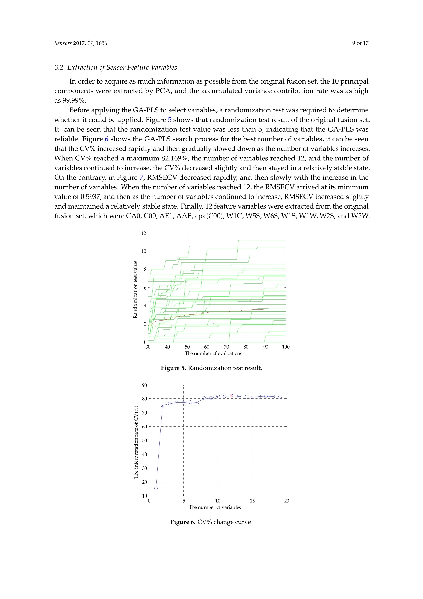
还剩15页未读,是否继续阅读?

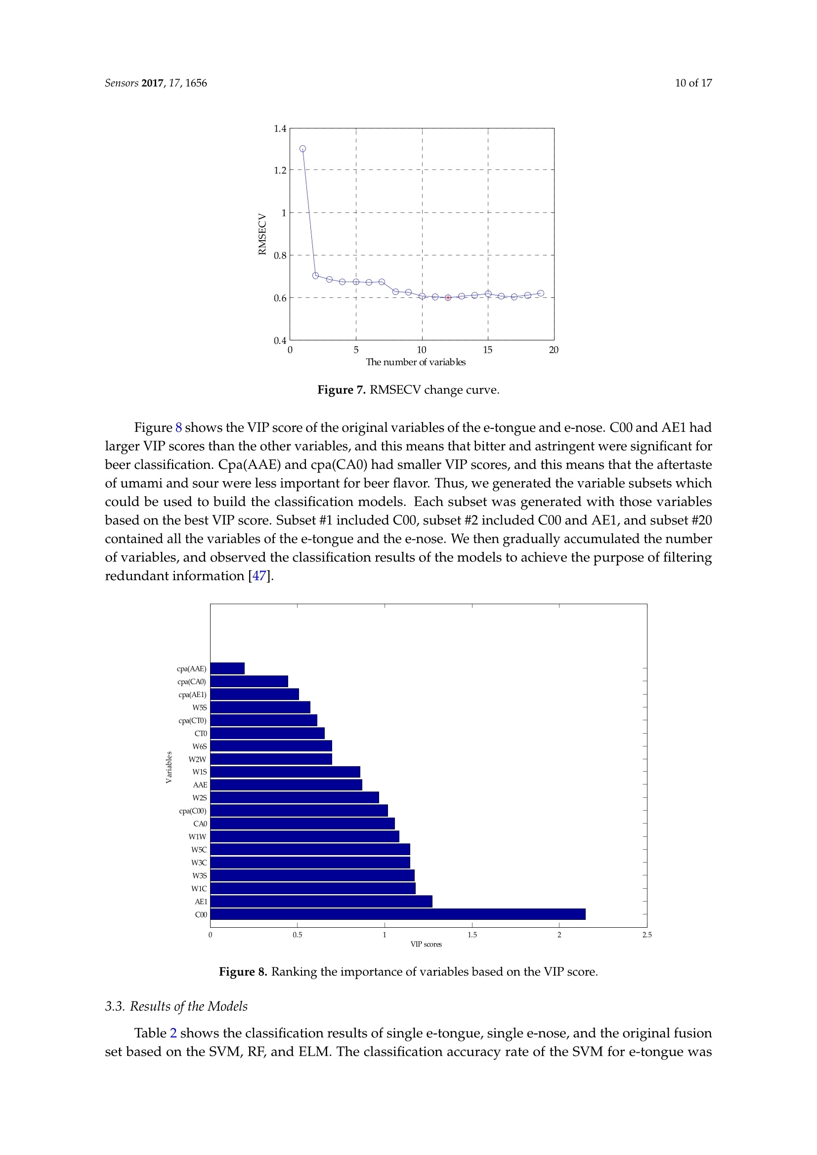
产品配置单

北京盈盛恒泰科技有限责任公司为您提供《啤酒中风味和滋味信息检测方案(感官智能分析)》,该方案主要用于啤酒中营养成分检测,参考标准--,《啤酒中风味和滋味信息检测方案(感官智能分析)》用到的仪器有德国AIRSENSE品牌PEN3电子鼻
推荐专场
感官智能分析系统(电子鼻/电子舌)
相关方案
更多
该厂商其他方案
更多