7根杆束的流体-结构相互作用：用实验数据对比数值模拟

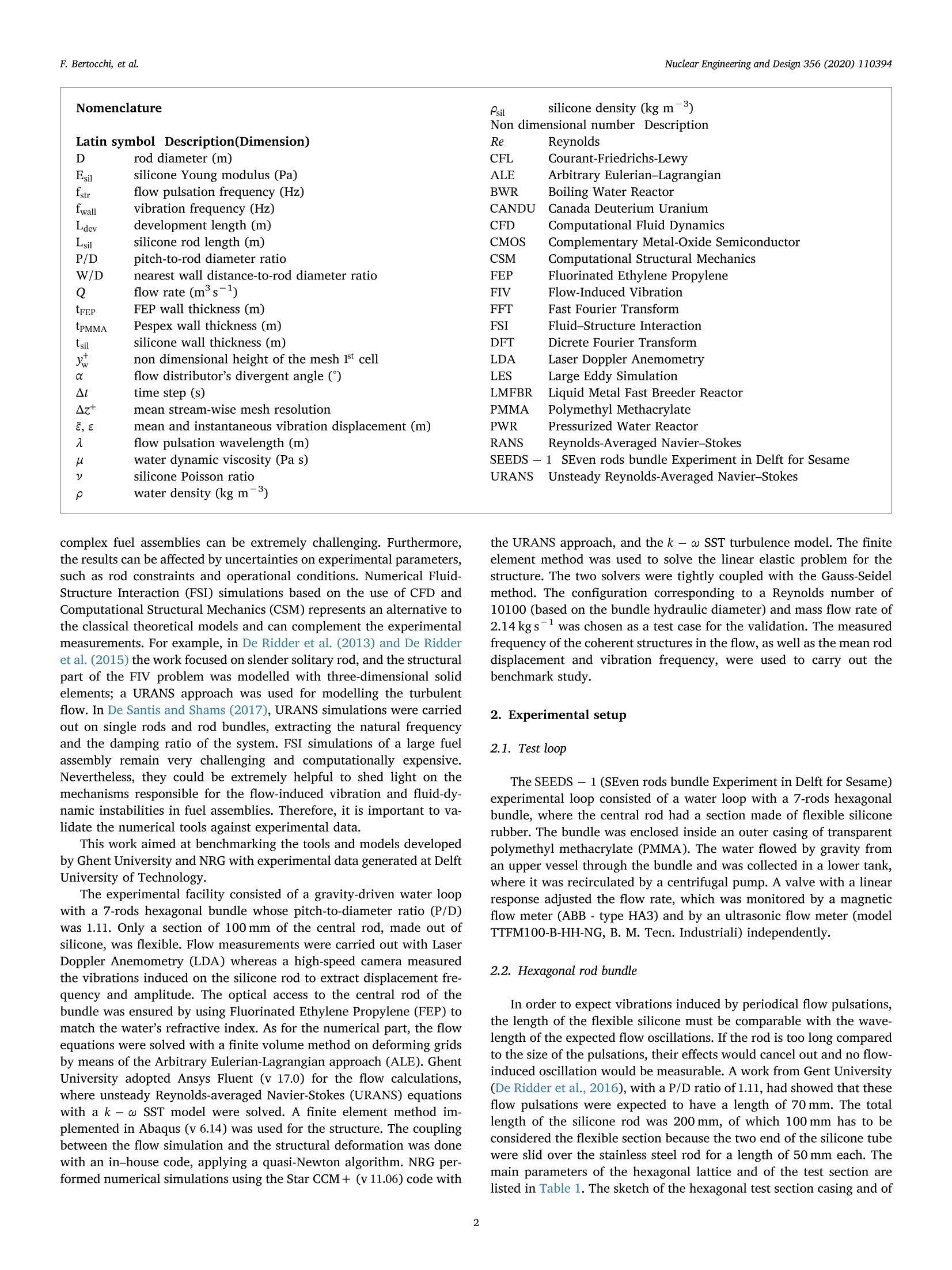
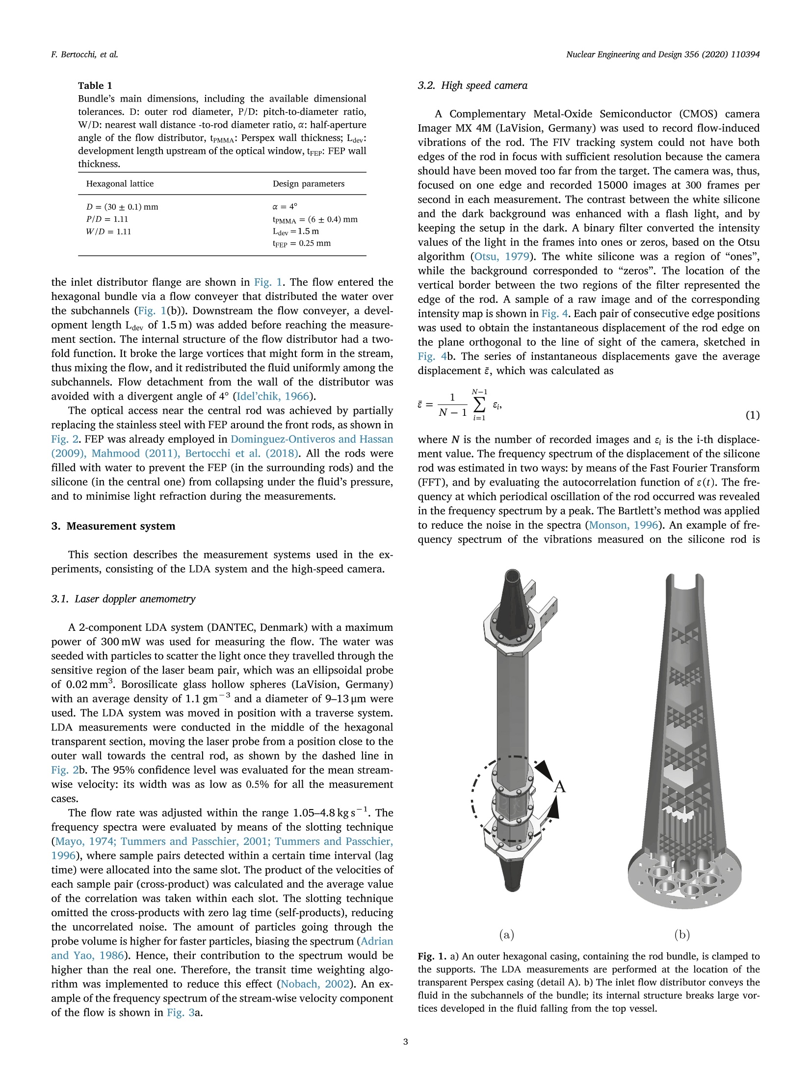
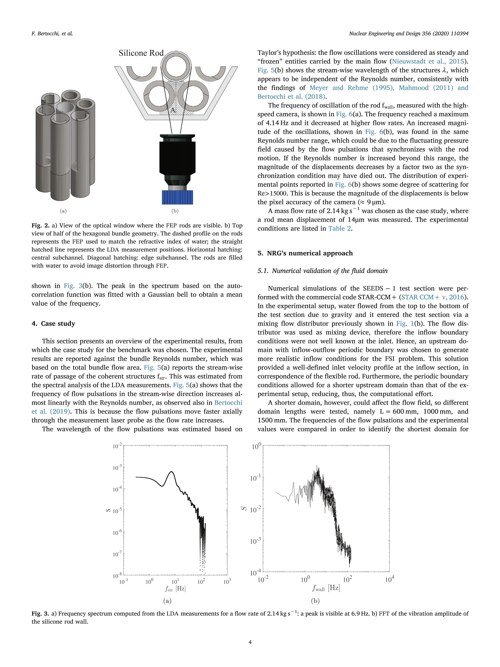
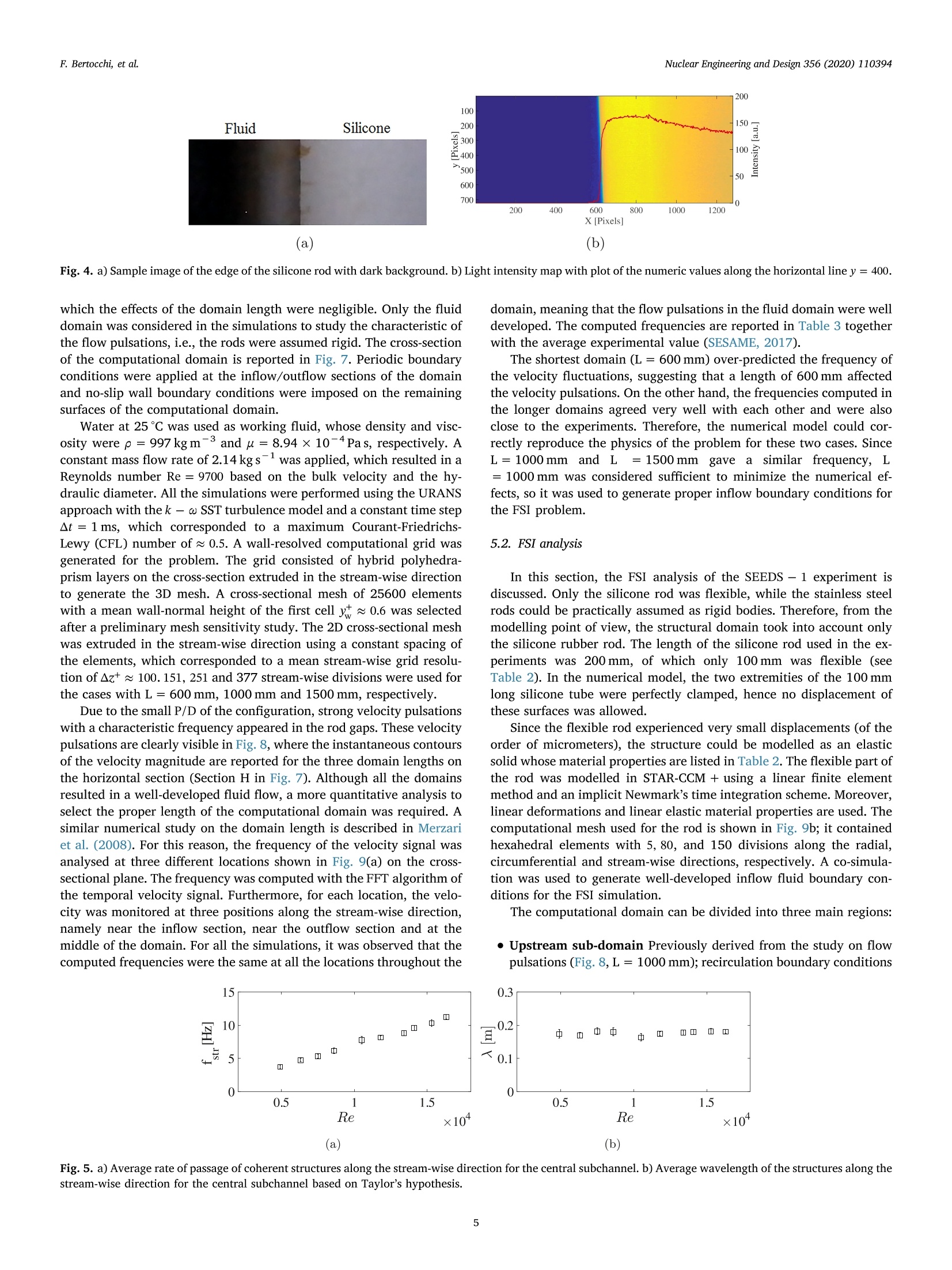
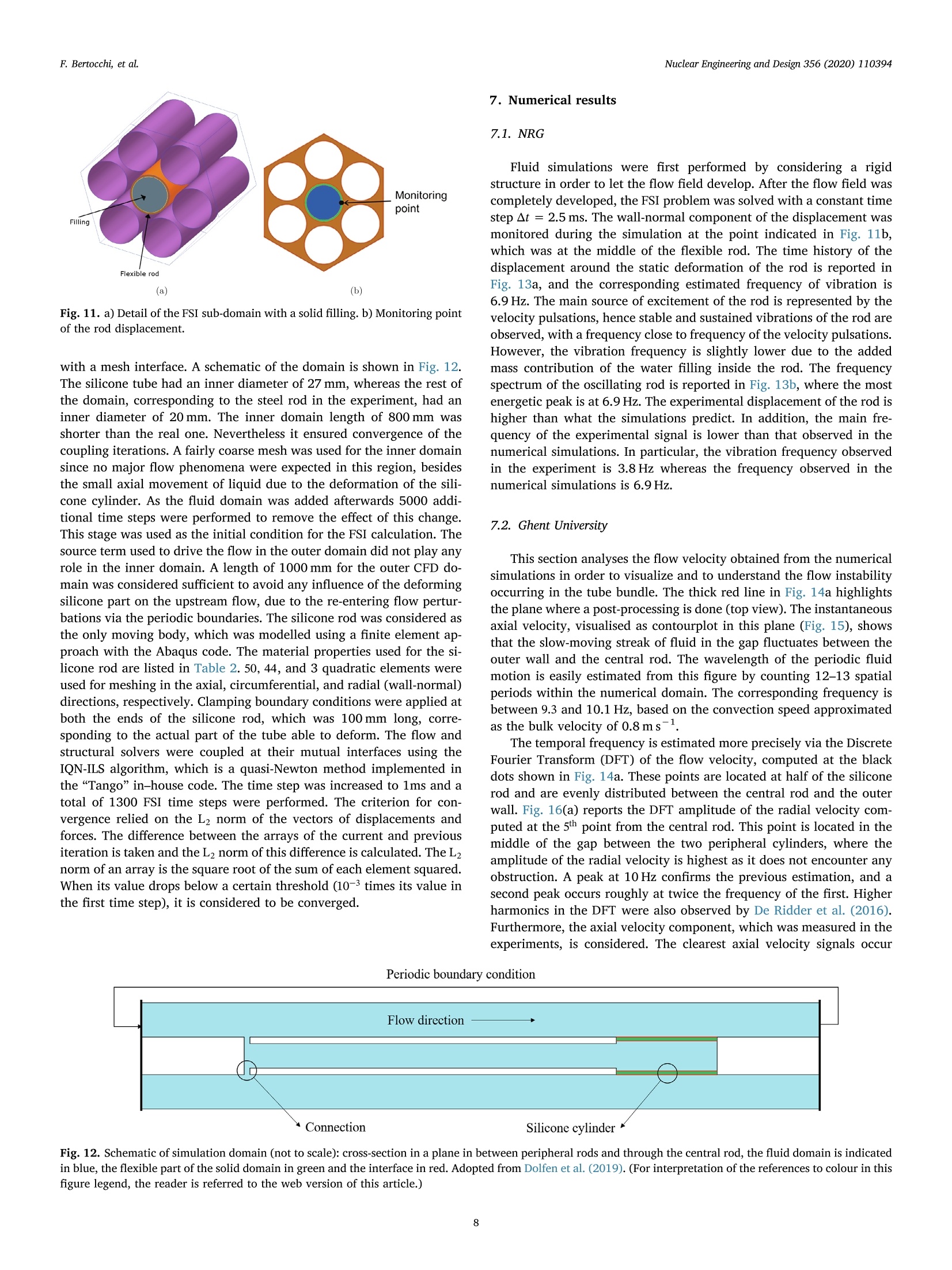
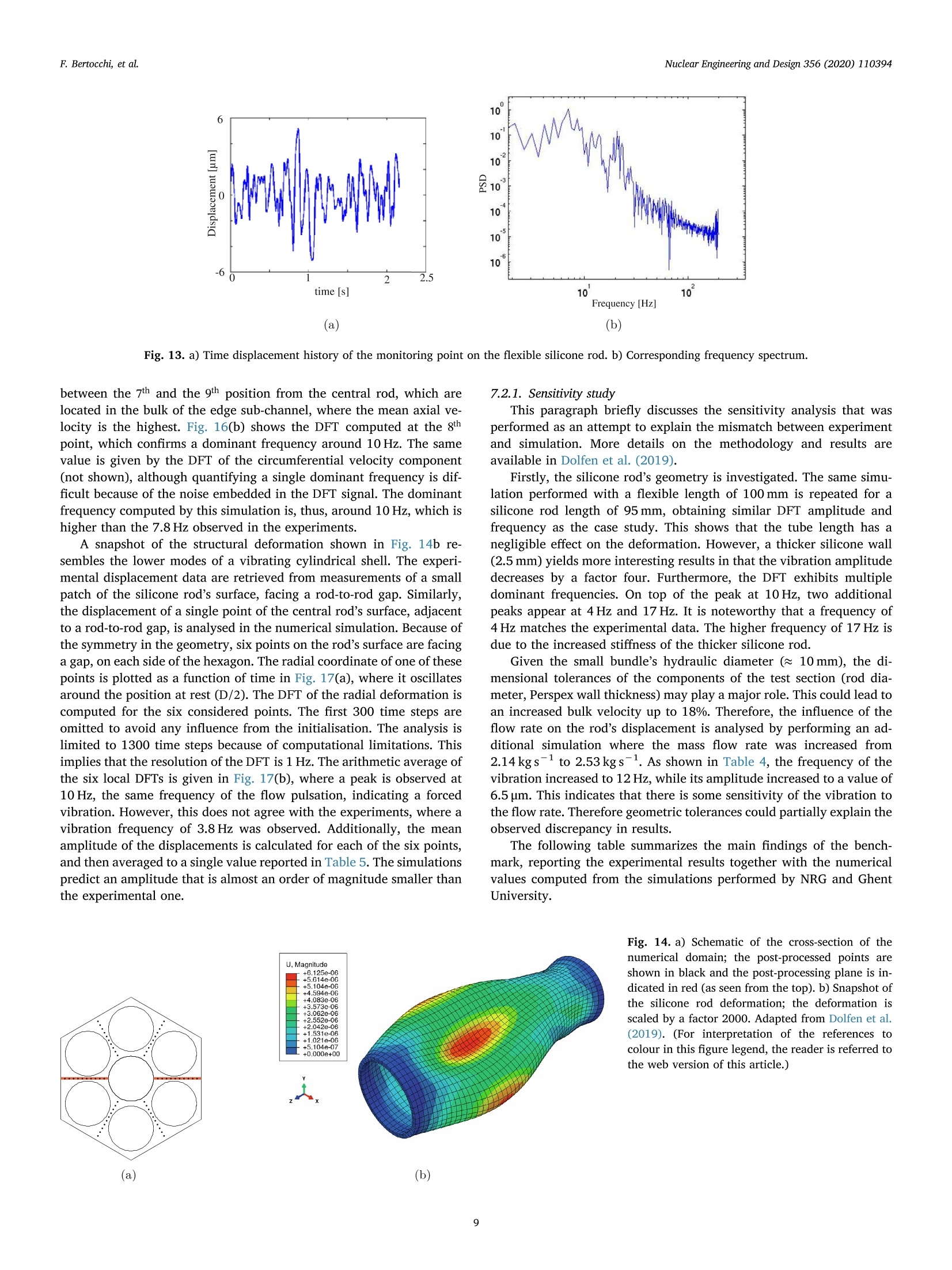
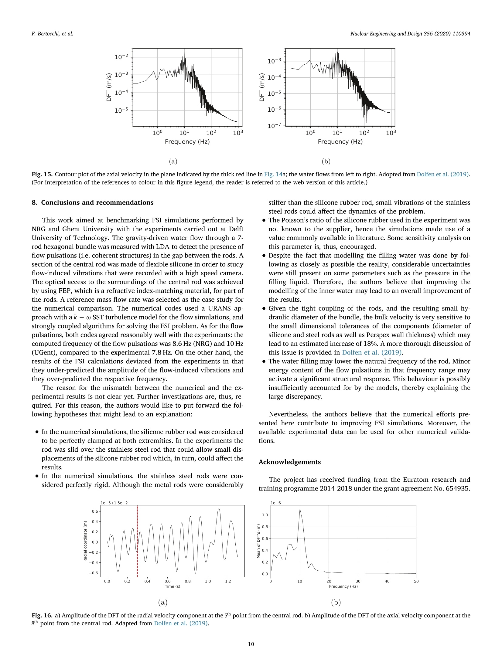
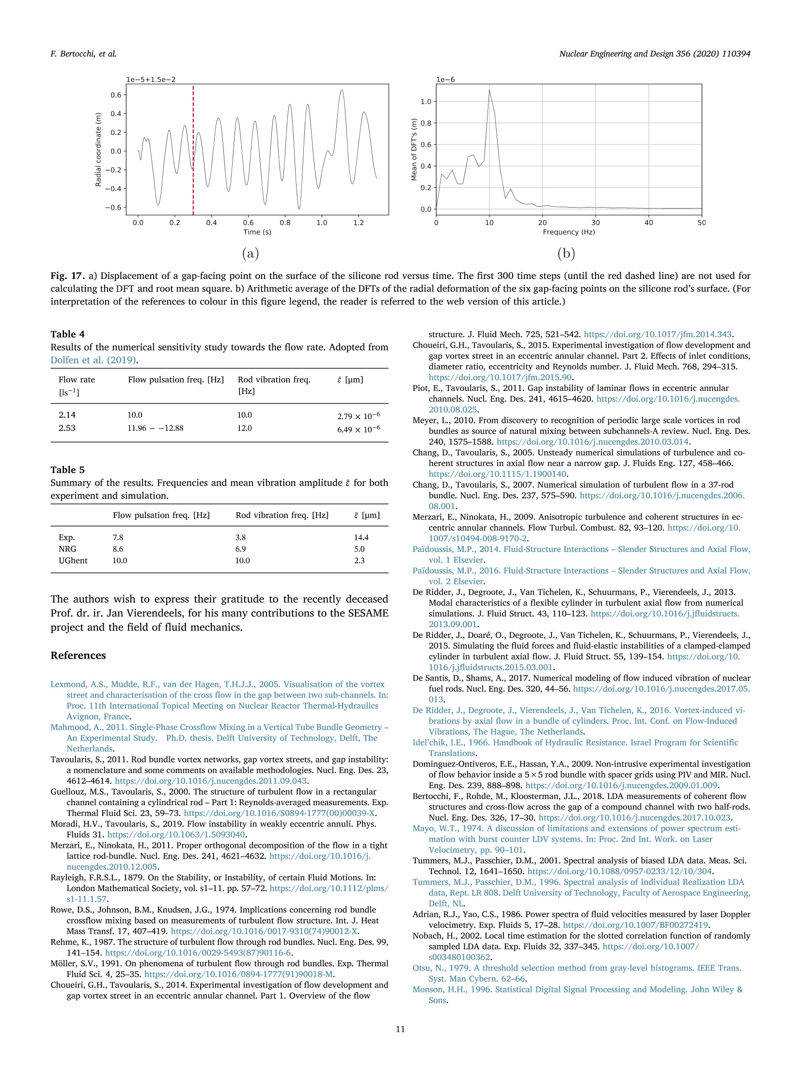
在核能应用中，棒束几何结构是非常常见的配置，可以在热交换器中、液态金属快中子繁殖反应堆(LMFBR)的堆芯、压水堆反应堆(PWR)、沸水反应堆(BWR)或加拿大重水反应堆(CANDU)中找到。当流体流经棒之间的空间时，低速区域与棒之间的速度差异会产生。这两个区域之间的剪切可能会触发由流体携带的大型相干结构条带 (Lexmond等人，2005；Mahmood，2011)，也称为间隙漩涡街。其形成机制尚未完全理解，有不同的理论已被提出。如果缝隙的速度分布具有拐点，则可能触发线性不稳定机制，正如Tavoularis（2011）、Guellouz和Tavoularis（2000）、Moradi和Tavoularis（2019）以及Merzari和Ninokata（2011）所讨论的那样，这将导致间隙漩涡街的形成。速度分布中的拐点被视为这些周期性漩涡形成的必要条件(尽管不充分)，正如Rayleigh的标准(Rayleigh, 1879)所预测的那样。过去(1974年的Rowe等人，1987年的Rehme，1991年的Möller)和最近(2014年和2015年的Choueiri和Tavoularis，2011年的Piot和Tavoularis)对棒束流中间隙漩涡街进行了许多实验。 Meyer(2010)对这个主题进行了广泛的回顾。由于计算机能力的提高，计算流体力学(CFD)研究也已被执行以研究这些现象。例如，一些最初的非稳态雷诺平均纳维尔-斯托克斯方程(URANS)模拟是由Chang和Tavoularis(2005)和Chang和Tavoularis(2007)执行的，而大涡模拟(LES)是由Merzari和Ninokata(2009)和Merzari和Ninokata(2011)执行的。间隙漩涡街可能会产生益处，因为它增强了燃料棒和核冷却剂之间的热交换，从而防止了燃料元件外包层的热点问题。Nuclear Engineering and Design 356 (2020) 110394 F. Bertocchi， et al.Nuclear Engineering and Design 356 (2020) 110394 Contents lists available at ScienceDirect Nuclear Engineering and Design journal homepage： www.elsevier.com/locate/nucengdes Fluid-structure interaction of a 7-rods bundle： Benchmarking numerical simulations with experimental data F. Bertocchi *， M. Rohde， D. De Santis， A. Shams ， H. Dolfen ， J. Degroote d ， J. Vierendeels a Faculty of Applied Sciences ， Department of Radiation Science and Technology， Delft University of Technology， Mekelweg 15， 2629 JB Delft， The Netherlands b Nuclear Research and Consultancy Group (NRG)， Westerduinweg 3， 1755 LE Petten， The Netherlands S Department of Flow， Heat and Combustion Mechanics， Ghent University， Sint-Pieternieuwstraat 41， B-9000 Ghent， Belgium d Flanders Make， Belgium ABSTRACT Fluid f lows through rod bundles are observed in many nuclear appl i cations， such as in the core of Gen IV liquid me t al fast breeder nuclear reactors (LMFBR). One of the main features of this configurat i on is t he appearance of flow fluctuations i n the rod gaps due to the velocity difference in t he sub-channels between the rods. On one side， these pulsations are beneficial as they enhance the heat exchange between the rods and the fluid. On the other side， the f l uid pulsations might induce vibrations of the flexible fuel rods， a mechanism generally referred to as Flow Induced Vibrations (F I V). Over t ime， this might result i n mechanical f atigue of t he r ods and rod fret t ing， which eventually can compromise their st r uctural i ntegri t y. Within t he SESAME framework， a joint work between Delft University of Technology (TU Delft)， Ghent University (UGent)， and NRG has been carried out with the aim of performing experimental measurements of FIV i n a 7-rods bundle and validate numerical simulations against the obtained experimenta l data. The experiments performed by TU Del f t consisted of a gravity-driven flow through a 7-rods， hexagonal bundle with a pitch-to-diameter ratio P/D= 1.11. A sect i on of 200 mm of the central rod was made out of si l icone， of which 100 mm were flexible. Flow mea-surements have been carried out with Laser Doppler Anemometry (LDA) whereas a high-speed camera has measured the v i brations i nduced on t he silicone rod. The numerical simulations made use of the Unsteady Reynolds-averaged Navier-Stokes equations (URANS) approach for the t urbulence modelling， and of strongly coupled algorithms for the solution of the fluid-structure i nteraction (FSI) problems. The measured frequency of the flow pulsations， as well as the mean rod displacement and vibration f requency， have been used to carry out the benchmark. 1. Introduction In nuclear applications， rod bundle geometries are very common configurations which can be found in heat exchangers， in the core of Liquid Metal Fast Breeder Reactors (LMFBR)， Pressurized Water Reactors (PWR)， Boil i ng Water Reactors (BWR) or Canadian Deuterium reactors (CANDU). When a fluid flows in the space between the rods， a velocity di f ference between the low-speed region in the rod gap and the bulk occurs. The shear between these two regions can trigger streaks of large coherent structures carried by the flow (L exmond et al.， 2005；Mahmood， 2011)， also known as gap vortex streets. The mechanism responsibl e for their formation i s not yet f ully understood， and different theories have been proposed. If t he velocity profile across t he gap has an inflection point， a l inear instability mechanism may be triggered， as discussed in Tavoular i s (2011)， Guellouz and Tavoularis (2000)， Moradi and Tavoularis (2019) and Merzari and Ni n okata (2011)， which leads to the formation of the gap vortex streets. The inflection point i n the ve-locity profile is regarded as a necessary (although not sufficient) con-dition for these periodical vortices to form， as predicted by the Ray-leigh ’s criterion (Rayle igh ， 1879). Many experiments on gap vortex streets in rod bundle flows have been done in the past (Rowe et al .，1974； Rehme， 1987； Mol l er ， 1991) and recently (C houei r i and Tavoularis， 2014； Choueiri and Tavoularis， 2015； Piot and Tavoul a ris，2011). An extensive review on the subject was provided by M eyer (2010). Because of the i ncrease in computer power， Computational Fluid Dynamics (CFD) studies have also been performed to study these phenomena. For example， some of the first Unsteady Reynolds-aver-aged Navier-Stokes equations (URANS) simulations were performed by Chang and T avoulari s (2005) and Chang and Tavoular i s (2007) and Large Eddy Simulations (LES) were performed by M erzari and Ninokata (2009) and Merzari and N i nokata (2011). The gap vortex streets can be beneficial due to the enhanced heat exchange between fuel rods and nuclear coolant ， which prevents hot spot s on the outer cladding of the fuel elements. However ， the vortex streets can be responsible for flow-induced vibration (FIV) which can cause wear， rod failure and fuel l eakage. I n the past few decades， t he study of FIV of slender bodies in axial flow has relied on simplified analytical models； a review of such models was provided by P aidoussi s (2014) and Paidoussis (2016). From t he ex-perimental point of view， measuring the small rod vibrations in E-mail address： F.Ber t occhi@tudel f t .nl (F. Ber t occhi). https：//doi.org/10.1016/j .nucengdes.2019.110394 Received 9 May 2019； Received i n revised f orm 18 September 2019； Accepted 21 October 2019 0029-5493/C 2019 The Authors. Published by Elsevier B.V. This is an open access article under the CC BY-NC-ND l icense Nomenclature Psil silicone density (kg m-3) Non dimensional number Description Latin symbol Description(Dimension) Re Reynolds D rod diameter (m) CFL Courant-Friedrichs-Lewy Esil silicone Young modulus (Pa) ALE Arbitrary Eulerian-Lagrangian fstr flow pulsation frequency (Hz) BWR Boiling Water Reactor fwall vibration frequency (Hz) CANDU Canada Deuterium Uranium Ldev development length (m) CFD Computational Fluid Dynamics Lsil silicone rod length (m) CMOS Complementary Metal-Oxide Semiconductor P/D pitch-to-rod diameter ratio CSM Computational Structural Mechanics W/D nearest wall distance-to-rod diameter ratio FEP Fluorinated Ethylene Propylene Q flow rate (m’s-1) FIV Flow-Induced Vibration tFEP FEP wall thickness (m) FFT Fast Fourier Transform tPMMA Pespex wall thickness (m) FSI Fluid-Structure Interaction tsil silicone wall thickness (m) DFT Dicrete Fourier Transform non dimensional height of the mesh ft cell LDA Laser Doppler Anemometry C flow distributor’s divergent angle (°) LES Large Eddy Simulation At time step (s) LMFBR Liquid Metal Fast Breeder Reactor Az+ mean stream-wise mesh resolution PMMA Polymethyl Methacrylate E，E mean and instantaneous vibration displacement (m) PWR Pressurized Water Reactor 入 flow pulsation wavelength (m) RANS Reynolds-Averaged Navier-Stokes water dynamic viscosity (Pa s) SEEDS - 1 SEven rods bundle Experiment in Delft for Sesame silicone Poisson ratio URANS Unsteady Reynolds-Averaged Navier-Stokes P water density (kg m-3) complex fuel assemblies can be extremely challenging. Furthermore，the results can be affected by uncertainties on experimental parameters，such as rod constraints and operational conditions. Numerical Fluid-Structure Interaction (FSI) simulations based on the use of CFD and Computational Structura l Mechanics (CSM) represents an alternative to the classical theoretical models and can complement t he experimental measurements. For example， in De Ridder et al. (2013) and De R idder e t al . (2015) the work focused on slender solitary rod， a nd the structural part of the FIV problem was modelled with three-dimensional solid elements； a URANS approach was used for modelling the turbulent flow. In De Santis and Shams (2017)， URANS simulations were carried out on single rods and rod bundles， extracting the natural frequency and the damping ratio of the system. FSI simulations of a large fuel assembly remain very challenging and computationally expensive.Nevertheless， they could be extremely helpful to shed l ight on the mechanisms responsible for the flow-induced vibration and fluid-dy-namic i nstabil i ties in fuel assemblies. Therefore， it is important to va-l i date the numerical tools against experimental data. This work aimed at benchmarking the tools and models developed by Ghent University and NRG with experimental data generated a t Del f t University of Technology. The exper i mental facility consisted of a gravity-driven water loop with a 7-rods hexagonal bundle whose pitch-to-diameter ratio (P/D)was 1.11. Only a section of 100 mm of the central rod， made out of silicone， was flexible. Flow measurements were carried out with Laser Doppler Anemometry (LDA) whereas a high-speed camera measured the vibrations induced on the silicone rod to extract displacement fre-quency and amplitude. The optical access to the central rod of the bundle was ensured by using Fluorinated Ethylene Propylene (FEP) to match the water’s refractive i ndex. As f or the numerical part， t he f low equations were solved with a finite volume method on deforming grids by means of the Arbitrary Eulerian-Lagrangian approach (ALE). Ghent University adopted Ansys Fluent (v 17.0) f or the flow calculations，where unsteady Reynolds-averaged Navier-Stokes (URANS) equations with a k -w SST model were solved. A finite element method im-plemented in Abaqus (v 6.14) was used for the structure. T he coupling between the flow simulation and the structural deformation was done with an in-house code， applying a quasi-Newton algorithm. NRG per-formed numerical simulations using the Star CCM+ (v11.06) code wi t h the URANS approach， and t he k - ω SST turbulence model. T he f i nite element method was used to solve the linear elastic problem for the structure. The t wo solvers were tightly coupled with the Gauss-Seidel method. The configuration corresponding to a Reynolds number of 10100 (based on the bundle hydraulic diameter) and mass flow r ate of 2.14 kg s-l was chosen as a test case for the validation. The measured frequency of the coherent structures in the flow， as well as the mean rod displacement and vibration frequency， were used to carry out the benchmark study. 2. Experimental setup 2.1. Test loop The SEEDS - 1 (SEven rods bundle Experiment in Delft for Sesame)experimental loop consisted of a water loop with a 7-rods hexagonal bundle， where the central rod had a section made of flexible si l icone rubber. The bundle was enclosed inside an outer casing of t ransparent polymethyl methacrylate (PMMA). The water f lowed by gravity from an upper vessel through the bundle and was collected in a lower tank，where i t was recirculated by a centrifugal pump. A valve with a linear response adjusted the f l ow rate， which was monitored by a magnetic flow meter (ABB -type HA3) and by an ultrasonic flow meter (model TTFM100-B-HH-NG， B. M. Tecn. Industrial i ) independently. 2.2. Hexagonal rod bundle I n order to expect vibrat i ons i nduced by periodical f l ow pul s ations，the length of the flexible silicone must be comparable with the wave-length of the expected flow oscillations. If the rod i s t oo l ong compared t o the size of the pulsations， their effects would cancel out and no f low-induced oscillation would be measurable. A work f rom Gent University (De Ridder et a l.， 2016)， with a P/D ratio of 1.11， had showed tha t these flow pulsations were expected to have a length of 70 mm. The total length of the silicone rod was 200 mm， of which 100 mm has t o be considered the flexible section because the two end of the silicone t ube were slid over the stainless steel rod for a length of 50 mm each. The main parameters of the hexagonal l at t ice and of the t est section are l i sted in Table 1. The sketch of the hexagonal test section casing and of Bundle’s main dimensions， including the available dimensional tolerances. D： outer rod diameter， P/D： pitch-to-diameter ratio，W/D： nearest wal l distance -to-rod diameter ratio， c： hal f -aperture angle of the flow distributor， tpMMA： Perspex wall thickness； Ldev：development l ength upstream of the optica l window， t FE p ： FEP wall thickness. Hexagonal lattice Design parameters D=(30±0.1)mm α=4° P/D=1.11 W/D=1.11 tPMMA=(6±0.4)mm Ldev=1.5 m tFEP = 0.25 mm the inlet distributor flange are shown i n Fi g. 1. The flow entered the hexagonal bundle via a f low conveyer that distributed the water over the subchannels (Fi g. 1(b)). Downstream t he f low conveyer， a devel -opment length Ldey of 1.5 m) was added before reaching the measure-ment section. The internal structure of the flow distributor had a two-fold function. It broke the large vortices t hat might form in t he stream，thus mixing the flow， and it redistributed the f luid uniformly among the subchannels. Flow detachment from the wall of the distributor was avoided with a divergent angle of 4° (I del ’chik， 1966). The optical access near the central rod was achieved by partially replacing the stainless steel with FEP around t he front rods， as shown in Fi g . 2. FEP was already employed i n Doming u ez-Ont i veros and H assan (2009)， Mahmood (2011)， B ertocchi e t al . (2018). All the rods were filled with water to prevent the FEP (i n the surrounding rods) and the si l icone (in the central one) from collapsing under the fluid’s pressure，and to minimise light refraction during the measurement s . 3. Measurement system This section describes the measurement systems used in the ex-periments， consist i ng of t he LDA system and the high-speed camera. 3.1. Laser doppler anemometry A 2-component LDA system (DANTEC， Denmark) with a maximum power of 300 mW was used for measuring the flow. The water was seeded with particles to scatter the l ight once they travel l ed through the sensitive region of t he laser beam pair， which was an ellipsoidal probe of 0.02 mm. Borosilicate glass hollow spheres (LaVision， Germany)with an average density of 1.1 gm-3 and a diameter of 9-13 um were used. The LDA system was moved in position with a traverse system.LDA measurements were conducted in the middle of the hexagonal transparent section， moving the laser probe from a posi t ion close to the outer wal l towards the central rod， as shown by the dashed l ine i n Fi g. 2b. The 95% confidence level was evaluated for the mean stream-wise velocity： its width was as low as 0.5% for al l the measurement cases. The f l ow rate was adjusted within the range 1.05-4.8 kgs -1. The frequency spectra were evaluated by means of the slotting technique (Mayo， 1974； Tummers and Pa s schier， 2001； Tummers and Passchier，1996)， where sample pairs detected within a certain t i me interval (lag time) were allocated into the same slot. The product of the velocities of each sample pair (cross-product) was calculated and the average value of the correlation was taken within each slot . The slotting technique omitted the cross-products with zero l ag time (self-products)， reducing the uncorrelated noise . The amount of particles going through the probe volume is higher for f aster particles， biasing the spectrum (Adrian and Yao， 1986). Hence， their contribution to the spectrum would be higher than the real one. Therefore， t he transit time weighting algo-rithm was implemented to reduce this effect (N obach， 2002). An ex-ample of the frequency spectrum of the stream-wise velocity component of the flow i s shown in Fig . 3a. A Complementary Metal-Oxide Semiconductor (CMOS) camera Imager MX 4M (LaVision， Germany) was used to record flow-induced vibrations of the rod. T he FIV tracking system could not have both edges of the rod in focus with sufficient resolution because the camera should have been moved too far from the target. The camera was， t hus，focused on one edge and recorded 15000 images at 300 f rames per second in each measurement . The contrast between the white silicone and the dark background was enhanced wi t h a flash l ight， and by keeping the setup in the dark. A binary filter converted t he i ntensity values of the light in the frames into ones or zeros， based on the Otsu algorithm (Otsu， 1979). The white silicone was a region of “ones”while the background corresponded to “zeros". The location of the vertical border between the two regions of the filter represented the edge of the rod. A sample of a raw i mage and of the corresponding intensity map is shown in Fig. 4. Each pai r of consecut i ve edge positions was used to obtain the instantaneous displacement of the rod edge on the plane orthogonal to the line of sight of the camera， sketched in Fig. 4b. The series of instantaneous displacements gave the average displacement E， which was calculated as where N i s the number of recorded images and e is the i -th displace-ment value. The frequency spectrum of the displacement of the silicone rod was est i mated in two ways： by means of the Fast Fourier Transform (FFT)， and by evaluating the autocorrelation function of e(t ). The f re-quency at which periodical osci l lation of the rod occurred was revealed in the f requency spectrum by a peak. T he Bartlett’s method was applied to reduce the noise in the spectra (Monson， 1996). An example of fre-quency spectrum of the vibrations measured on the silicone rod is (a) (b) Fig. 1. a) An outer hexagonal casing， containing the rod bundle， i s clamped to the supports. The LDA measurements are performed at the location of the transparent Perspex casing (detail A). b) The inlet f low distributor conveys the f luid in the subchannels of the bundle； i ts internal structure breaks large vor-tices developed in the f l uid f all i ng from t he top vesse l. (a ) (b ) Fig. 2. a) View of the optical window where the FEP rods are v i sible. b) Top view of hal f of the hexagonal bundle geometry. The dashed profile on t he rods represents the FEP used to match the refractive index of water； the straight hatched l ine represents the LDA measurement positions. Horizontal hatching：central subchannel . Diagonal hatching： edge subchannel. The rods are filled with water to avoid image distortion through FEP. shown in Fig . 3(b). The peak in t he spectrum based on the auto-correlation function was fitted with a Gaussian bell to obtain a mean value of the frequency. 4. Case study This section presents an overview of the experimental results， from which the case study for the benchmark was chosen. The experimental results are reported against the bundle Reynolds number， which was based on the total bundle flow area. F ig. 5(a) r eports t he stream-wise rate of passage of the coherent structures fs t r. This was estimated from the spectra l analysis of the LDA measurements. Fi g.5(a) shows tha t the frequency of flow pulsations in the stream-wise direction increases al-most l inearly with the Reynolds number， as observed also in Bertocchi et al. (2019). This is because t he flow pulsations move faster axially through the measurement laser probe as the f low rate i ncreases. The wavelength of the flow pulsat i ons was estimated based on Taylor’s hypothesis： t he flow osci l lations were considered as steady and “frozen”entit i es carried by the main flow (N i e uwstadt e t al.， 2015).Fig.5(b) shows the stream-wise wavelength of the structures 入， which appears to be independent of t he Reynolds number， consistently with the findings of Meyer and Rehme (1995)， Mahmood (2011) and Bertocchi et al. (2018). The frequency of oscillation of the rod f wall ， measured with the high-speed camera， is shown in F ig.6(a). The f requency reached a maximum of 4.14 Hz and it decreased at higher flow rates. An i ncreased magni -tude of the oscillations， shown in F ig. 6(b)， was found in t he same Reynolds number range ， which could be due to the fluctuating pressure field caused by the flow pulsations that synchronizes wi t h the rod motion. If the Reynolds number is increased beyond this range， the magnitude of the displacements decreases by a factor two as the syn-chronization condition may have died out. The dist r ibution of experi -mental points reported in F ig. 6(b) shows some degree of scattering for Re>15000. This is because the magnitude of t he displacements is below the pixel accuracy of the camera (≈ 9um). A mass f low r ate of 2.14 kg s -1 was chosen as the case study， where a rod mean displacement of 14um was measured. The experimental conditions are listed in T able 2. 5. NRG's numerical approach 5.1. Numerical validation of the fluid domain Numerical simulations of the SEEDS - 1 test section were per-formed with the commercial code STAR-CCM+ (STAR CCM + v， 2016).In the experimental setup， water f lowed from the top to t he bottom of the test section due to gravity and it entered t he test section via a mixing flow distributor previously shown i n Fig. 1(b). The flow dis-tributor was used as mixing device， therefore the i nflow boundary conditions were not wel l known at the inlet. Hence， an upstream do-main with inflow-outflow periodic boundary was chosen t o generate more realistic inflow conditions for the FSI problem. This solution provided a well-defined inlet velocity profile at the inflow sect i on， i n correspondence of the f lexible rod. Furthermore， t he periodic boundary conditions allowed for a shorter upstream domain than that of the ex-per i mental setup， reduc i ng， thus， the computational effort. A shorter domain， however， could affect the flow f i eld， so different domain lengths were tested， namely L=600 mm， 1000mm， and 1500 mm. The frequencies of the flow pulsations and t he experimental values were compared in order to ident i fy the shortest domain for Fig. 3. a) Frequency spectrum computed from t he LDA measurements f or a f low rat e of 2.14 kg s-1： a peak i s visible at 6.9 Hz. b) FFT of the vibration amplitude of the silicone rod wall. which the effects of the domain length were negligible. Only the fluid domain was considered in the simulations to study the characteristic of the f low pulsations， i .e.， the rods were assumed rigid. The cross-section of the computational domain is reported in Fi g. 7. Periodic boundary conditions were appl i ed at the inf l ow/outf l ow sections of t he domain and no-slip wal l boundary conditions were imposed on the remaining surfaces of the computational domain. Water at 25℃ was used as working fluid， whose density and visc-osity were p = 997 kg m-3and p=8.94 × 10-4Pa s， respectively. A constant mass f low rate of 2.14 kg s - was applied， which resulted i n a Reynolds number Re =9700 based on the bulk velocity and the hy-draulic diameter. All the simulations were performed using the URANS approach with the k - w SST turbulence model and a constant time step At =1 ms， which corresponded to a maximum Courant-Friedrichs-Lewy (CFL) number of ~0.5. A wall-resolved computat i onal grid was generated for the problem. The grid consisted of hybrid polyhedra-prism layers on the cross-section extruded in the stream-wise direction to generate the 3D mesh. A cross-sectional mesh of 25600 elements with a mean wall-normal height of the first cell y~0.6 was selected after a prel i minary mesh sensi t ivity study. The 2D cross-sectional mesh was extruded in the stream-wise direction using a constant spacing of the elements， which corresponded to a mean stream-wise grid resolu-tion of Az+≈ 100.151，251 and 377 stream-wise divisions were used for the cases with L = 600 mm， 1000 mm and 1500 mm， respectively. Due to the small P/D of the configuration， strong velocity pulsat i ons with a characteristic frequency appeared in t he rod gaps. These velocity pulsations are clearly visible i n F i g. 8， where the i nstantaneous contours of the velocity magni t ude are reported f or the three domain l engths on the horizontal section (Section H in Fig. 7). Although all the domains resulted in a wel l -developed fluid flow， a more quantitative analysis to select the proper length of the computational domain was required. A similar numerical study on the domain length is described in Merzari et al . (2008). For this reason， the frequency of the velocity signal was analysed at three different locations shown in Fi g. 9(a) on the cross-sectional plane. The frequency was computed wi t h the FFT algori t hm of the temporal velocity signal. Furthermore， for eac h location， the velo-city was monitored at three posi t ions along the stream-wise direction，namely near the inflow section， near the outflow section and at the middle of t he domain. For all the simulations， it was observed that the computed frequencies were the same at all the locations t hroughout the domain， meaning that the flow pulsations in the fluid domain were well developed. The computed frequencies are reported in T a ble 3 together with the average experimental value (SESAME ， 2017). The shortest domain (L = 600 mm) over-predicted the frequency of the veloci t y fluctuations， suggesting that a length of 600 mm affected the velocity pulsations. On the other hand， the frequencies computed i n the longer domains agreed very wel l with each other and were also close to the experiments. Therefore， the numerical model could cor-rectly reproduce the physics of t he problem for these t wo cases. Since L=1000mm and L =1500 mm gave a similar frequency， L =1000 mm was considered sufficient to minimize t he numerical ef-fects， so i t was used to generate proper inflow boundary conditions for the FSI problem. 5.2. FSI analysis In this section， the FSI analysis of the SEEDS -1 experiment i s discussed. Only the sil i cone rod was flexible， while the stainless steel rods could be practically assumed as rigid bodies. Therefore， from the model li ng point of view， the structural domain took i nto account only the silicone rubber rod. The length of the silicone rod used in the ex-periments was 200 mm， of which only 100 mm was flexible (see Table 2). In the numer i cal model ， the two extremities of the 100 mm long si l icone tube were perfectly clamped， hence no displacement of these surfaces was allowed. Since the flexible rod experienced very small displacements (of the order of micrometers)， the structure could be modelled as an elastic solid whose material properties are listed in Table 2. The flexible part of the rod was modelled in STAR-CCM + using a linear fini t e element method and an implicit Newmark's time i ntegration scheme. Moreover，linear deformations and l i near elastic material propert i es are used. The computational mesh used for the rod is shown in Fig . 9b； it contained hexahedral elements with 5， 80， and 150 divisions along the radial，circumferential and stream-wise directions， respectively. A co-simula-tion was used to generate well-developed i nflow f luid boundary con-ditions for the FSI simulation. The computational domain can be divided into three main regions： ·Upstream sub-domain Previously derived from the study on flow pulsations (F ig . 8，L=1000 mm)； recirculation boundary conditions Fig . 5. a) Average rate of passage of coherent structures along the stream-wise direction for t he central subchannel. b) Average wavelength of t he structures along t he stream-wise direction for the central subchannel based on Taylor’s hypothesis. (a) (b) Fig. 6. a) Response frequency and b) mean displacement of the rod against t he Reynolds number based on t he near-wal l subchannel f low area (edge subchannel). Table 2 Material properties of the silicone rod with dimensional tolerances， where available： Psi si l icone density， v Poisson’s ratio， Esil Young’s modulus， Lsil flexible length of silicone， t s il silicone rod wall thickness. Experimental condi-tions adopted as reference case： Q volumetric flow rate， Re Reynolds number，e mean displacement ， fwa l l frequency of oscillation of the rod， fstr frequency of coherent structures i n the axial direction. Silicone properties Experimental conditions Psil 1180kgm-3 2.14×10-3m³s-1 0.48 10100 1MPa 14um sil (100±5)mm f、fwall 3.8 Hz (1.5±1)mm fstr 7.8Hz (a ) Fig. 7. Cross-sec t ional view of computational grid t ogether with close up view around the rod gap. were applied， and only a fluid problem was solved. ·FSI sub-domain It included the f lexible rod， shown in more detail in F i g. 11. This sub-domain was 100 mm long and consisted of six r igid rods surrounding a f lexible one i n the centre. The velocity profile at the inlet section of the sub-domain was mapped from the outlet of the upstream sub-domain. No boundary condition was applied at the interface between the upstream and the FSI sub-domain. All the internal surfaces of the FSI section were treated as no-slip walls.Furthermore， the surface of the middle rod was treated as a flexible wal l and FSI compatibil i ty conditions were applied， while the re-maining walls were considered rigid. The cross-sectional fl uid mesh was the same used in the upstream recirculation sub-domain， while 87 subdivisions were used in the stream-wise direction， with a re-sulting stream-wise mesh resolution of Az+≈30. ·Outflow sub-domain It was 100 mm long and it r educed t he effects of the outlet boundary conditions on the solution of the FSI sub-domain. I t contained only rigid rods， hence onl y a fluid problem was solved. The inlet section was an internal interface， hence no boundary condition was imposed. On the other hand， a pressure outlet boundary condition was i mposed at the out f low section. The remaining surfaces of the sub-domain were treated as rigid walls.The cross-sectional fluid mesh was the same used in the upstream sub-domain， while in the stream-wise direction 20 subdivisions were used. In the experimental setup， the rods were f illed with stagnant water to prevent the sil i cone rod f rom col l apsing under the effect of the f l uid's external pressure. The numerical simulations initially considered the filling material of the central rod as a solid with properties similar to the water， and with the length of the f lexible portion of the silicone rod，whose scheme i s shown in F i g. 11a. However， this approach was abandoned since it introduced too many uncertainties on t he values of the material properties. Moreover， from preliminary FSI simulations， it was observed that it would considerably over-estimate t he r igidity of the rod. An alternative way of modelling the internal f l uid was then pursued. 5.2.1. Additional modelling of the filling A more realistic modelling of the f il l ing would take into account the actual fluid wi t hin the rod. For this reason， the computational domain was modified as in F ig . 10b. Thi s model and the one previously shown in Fig . 10a were similar except for the addi t ional f l uid domain added to account for the water fi l ling the central rod. This additional domain consisted of a cyl i nder of stagnant water at atmospheric pressure with a diameter of 27 mm (i.e. the i nner diameter of the si l icone rod) and length of 1980 mm (i .e. the length of the water column in t he experi -ments， including the downstream length). This choice was made i n order to keep the configuration as close as possible to the experiments and to avoid spurious pressure f luctuations between the two extremi t ies in the case of a short domain. The portion in contact with the inner wall of the flexible rod was assumed to be a deforming no-slip wall. The r emaining surfaces were considered as fixed no-slip walls. Due to the fact that t he f i lling fluid was displaced only by the small oscillations of t he si l icone rubber rod，the magnitude of the velocities expected within this domain was smal l .Therefore， a coarse mesh for the fill i ng was used to reduce the com-putational cost. The adopted cross-sectional mesh consisted of ap-proximately 500 polyhedrons with a prism layer near the wall； this mesh was then extruded in the stream-wise direction using 500 divi -sions . The materia l proper ti es of the fil l ing were t he same of water in Velocity： Magnitude (m/s) Fig. 8. Instantaneous velocity contours on the middle section (H) for different lengths of the domain. From top to bottom： L = 600 mm， 1000 mm and 1500mm. (a) (b) Fig. 9. a) Locations used to measure t he f requency of t he velocit y pulsat i ons. b)Structural mesh for the flexible silicone rubber rod. Table 3 Frequencies of the velocity pulsations computed with di f ferent l engths of the domain and average frequency measured i n the experiment. L=600mm L=1000mm L=1500mm Experimental 9.4 Hz 8.6Hz 8.5 Hz 7.8 Hz the main f luid domain. 6. Ghent University's numerical approach The numerical approach consisted of t wo parts： the first focused on s i mulat i ng the flow， and the second considered the f l uid-structure in-teraction. 6.1. Flow simulation The geometry of the experiment was f i rst created in a simplified form for CFD simulations. The Fluent CFD code with the finite volume method was used. The mesh was entirely built with hexahedral cells.Along the circumference of the cylinder， 120 divisions were used， 10div i sions in between two rods and 700 divisions in t he axial direction.The inlet and outlet of the domain were connected via periodic boundary condi t ions. A stream-wise pressure gradient， implemented as a source term in the axial momentum equation， was applied to drive the flow. This ensured a f ully developed f low throughout t he domain，avoiding a flow development region. The pressure gradient was de-termined by running several times the same simulation， and repeatedly correcting its value until the mass f low rate was within 1% of the de-sired value of 2.14 kg s-1. The final value was 935.7 Pa m-. A l ength of 100 mm was judged sufficient for this mesh， allowing enough vortex street wavelengths to develop. Since steady Reynolds-averaged Navier- Flow dire ction (a) Fig. 10. a) Computational domain used to performed FSI simulations. b) De t ail of the FSI sub-domain with the water-fil l ing domain. Stokes equations (RANS) simulations could not properly predict the f luctuating flow， a URANS approach was followed adopting a k -ω SST turbulence model， the same approach as chosen by NRG. It has been demonstrated multiple times in t he past t hat URANS is able to capture the gap vortex (De Ridde r e t al .， 2016). A time domain spanning 11 s was discretised into 20000 time steps of 0.55 ms. This corresponded to about 8.5 through-flows of the domain， based on t he bulk velocity. TheSev velocity components collected at several points in the domain are stored at every time step. After the simulation， this data were post-processed and the main frequencies were determined. 6.2. FSI analysis In the second part ， a fully coupled FSI simulation was set up. Since the central rod was a hollow tube filled with water， the CFD domain had first to be adapted. Therefore i t was closed at the bottom， and connected at the top to the outer domain via a short annular sect i on Fig. 11. a) Detail of the FSI sub-domain with a solid f i ll i ng. b) Monitor i ng point of the rod displacement. with a mesh interface. A schematic of the domain i s shown in F i g . 12.The s i licone tube had an inner diameter of 27 mm， whereas the rest of the domain， corresponding to the steel rod in the experiment ， had an inner diameter of 20 mm. The inner domain length of 800 mm was shorter than the real one. Nevertheless it ensured convergence of the coupling iterations. A fairly coarse mesh wa s used for the inner domain since no major flow phenomena were expected in this region， besides the smal l axial movement of liquid due to the deformation of the sil i -cone cyl i nder. As the fluid domain was added afterwards 5000 addi-tional time steps were performed to remove the effect of t his change.This stage was used as the initial condition for the FSI calculation. The source term used to drive the flow in the outer domain did not play any role in the inner domain. A length of 1000 mm for the outer CFD do-main was considered sufficient to avoid any influence of the deforming silicone part on the upstream flow， due to the re-entering flow pertur-bations via the periodic boundaries. The s i licone rod was considered as the only moving body， which was modelled using a finite element ap-proach wi t h the Abaqus code. The material properties used for t he si-licone rod are listed in Table 2. 50，44， and 3 quadratic elements were used for meshing in the axial ， circumferential ， and r adial (wall-normal)direc t ions， respectively. Clamping boundary condit i ons were applied at both the ends of the silicone rod， which was 100 mm long， corre-sponding to the actual part of the tube able to deform. The flow and structural solvers were coupled at their mutual interfaces using the IQN-ILS algorithm， which is a quasi-Newton method implemented in the“Tango”in-house code. The time step was increased to 1ms and a total of 1300 FSI time steps were performed. The criterion for con-vergence relied on the L2 norm of the vectors of displacements and forces. The difference between the arrays of the current and previous iteration is taken and the L2 norm of this difference is calculated. The L2norm of an array is the square root of the sum of each element squared.When its value drops below a certain threshold (10-3 times it s value in the first time step)， it is considered to be converged. 7.1. NRG Fluid simulations were first performed by considering a rigid structure in order to let the flow field develop. After the flow field was completely developed， the FSI problem was solved with a constant time step At =2.5 ms. The wall-normal component of the displacement was monitored during the simulation at the point indicated in Fig. 11b，which was at the middle of t he flexible rod. The t ime history of the displacement around the static deformation of the rod is reported in Fi g . 13a， and the corresponding est i mated frequency of vibration i s 6.9 Hz. The main source of excitement of the rod is represented by the velocity pulsations， hence stable and sustained vibrations of the r od are observed， with a frequency close to frequency of the velocity pulsations.However， the vibration frequency is sl i ghtly lower due to the added mass contribution of the water filling inside the rod. The frequency spectrum of the osci l lating rod is reported in Fig . 13b， where the most energetic peak is at 6.9 Hz. The experimental displacement of the rod i s higher than what the simulations predict. In addition， the main fre-quency of the experimental signal is l ower than that observed in the numerical simulations. In particular， the vibration frequency observed in the experiment is 3.8 Hz whereas the frequency observed i n the numerical simulat i ons is 6.9 Hz. 7.2. Ghent University This section analyses t he flow velocity obtained from the numerical simulations in order to visualize and to understand the flow instability occurring in the tube bundle. The thick red l ine i n F i g. 14a highl i ghts the plane where a post-processing is done (top view). The instantaneous axial velocity， visualised as contourplot in this plane (F i g. 15)， shows that the slow-moving streak of f luid i n the gap fluctuates between the outer wall and the central rod. The wavelength of the periodic f luid motion is easily est i mated from this figure by counting 12-13 spatial periods wi t hin the numerical domain. The corresponding frequency is between 9.3 and 10.1 Hz， based on the convection speed approximated as the bulk velocity of 0.8 ms -1. The temporal frequency is estimated more precisely via the Discrete Fourier Transform (DFT) of the flow velocity， computed at the black dot s shown in F ig . 14a. These points are located at half of the silicone rod and are evenly distributed between the central rod and t he outer wall . F i g. 16(a) reports the DFT amplitude of the radial velocity com-puted at the 5th point from the central rod. This point i s located i n the middle of the gap between the two peripheral cylinders， where the amplitude of the radial velocity is highest as it does not encounter any obstruction. A peak at 10 Hz confirms the previous estimation， and a second peak occurs roughly at twice t he f requency of t he f i rst. Higher harmonics in the DFT were also observed by D e Ridder et al. (2016).Furthermore， the axial velocity component， which was measured in the experiments， is considered. The clearest axial velocity signals occur Connection Silicone cylinder Fig. 12. Schematic of simulation domain (not to scale)： cross-section in a plane i n between peripheral r ods and t hrough the central rod， the f l uid domain is i ndicated in blue， the flexible part of the solid domain i n green and the i nterface in red. Adopted from Dolfen et al. (2019). (For interpretation of the r eferences to colour in this figure legend， the reader is referred to the web version of this article.) (a ) Fig. 13. a) Time displacement history of the monitor i ng point on the flexible si l icone rod. b) Corresponding frequency spectrum. between the 7th and the 9th position f rom the central rod， which are located in the bulk of the edge sub-channel， where the mean axial ve-locity is the highest . Fi g . 16(b) shows the DFT computed at the 8th point， which confirms a dominant frequency around 10 Hz. The same value is given by the DFT of the circumferential velocity component (not shown)， although quant i fying a single dominant f requency is dif-ficult because of the noise embedded in the DFT signal. The dominant frequency computed by this simulation is， thus， around 10 Hz， which is higher than the 7.8 Hz observed in t he experiments. A snapshot of the structural deformat i on shown i n Fig . 14b re-sembles the lower modes of a vibrating cylindrical shell . The experi-mental displacement data are retrieved f rom measurements of a small patch of the silicone rod’s surface， facing a r od-to-rod gap. Similarly，the displacement of a single point of t he central rod’s surface， adjacent to a rod-to-rod gap， is analysed in the numerical simulation. Because of the symmetry in the geometry， six points on the rod's surface are f acing a gap， on each side of the hexagon. The radial coordinate of one of t hese points is plotted as a function of time in Fi g. 17(a)， where i t oscillates around the position at r est (D/2). The DFT of the radial deformation is computed for the six considered points. The f i rst 300 t i me steps are omitted to avoid any influence from the ini ti alisation. The analysis is limited to 1300 time steps because of computational l imitations. T h is implies that t he resolution of the DFT i s 1 Hz. The ari t hmetic average of the six local DFTs is given in F ig. 17(b)， where a peak i s observed at 10 Hz， the same frequency of the flow pulsation， indicating a forced vibration. However ， this does not agree with the experiments， where a vibration frequency of 3.8 Hz was observed. Addi ti onal l y， the mean amplitude of the displacements is calculated for each of t he six point s ，and then averaged to a single value reported in Table 5. The simulations predict an ampl i tude that is almost an order of magnitude smaller than the experimental one. 7.2.1. Sensitivity study This paragraph briefly discusses the sensi t ivity analysis t hat was performed as an attempt to explain the mismatch between experiment and simulation . More details on t he methodology and resul t s are available in D o l fen et al . (2019). Firstly， the silicone rod’s geometry i s i nvestigated. The same simu-lation performed with a flexible length of 100 mm is repeated for a s il icone rod length of 95 mm， obtaining simi l ar DFT amplitude and frequency as the case study. This shows that the tube length has a negligible effect on the deformation. However， a thicker silicone wall (2.5 mm) yields more interesting results in that the vibration amplitude decreases by a factor four. Furthermore， the DF T exhibi t s multiple dominant frequencies. On top of the peak at 10 Hz， two additional peaks appear at 4 Hz and 17 Hz. I t is noteworthy that a frequency of 4 Hz matches the experimental data. The higher frequency of 17 Hz i s due to the increased sti f fness of the thicker silicone rod. Given the small bundle’s hydraulic diameter (~10mm)， the di-mensional tolerances of the components of the test section (rod dia-mete r ， Perspex wall thickness) may play a major role. This could lead to an i ncreased bulk velocity up to 18%. Therefore， the i nf l uence of the flow rate on the rod’s displacement i s analysed by performing an ad-ditional simulation where the mass flow rate was increased from 2.14kgs -l to 2.53 kg s -1. As shown i n T a ble 4， the frequency of the vibration increased to 12 Hz， while its amplitude increased to a value of 6.5 um. This indicates that there is some sensitivity of the vibration to the flow rate. Therefore geometric tolerances could partially explain the observed discrepancy i n results. The following table summarizes the main findings of the bench-mark， repor t ing the experimental results together with the numerical values computed from the simulations performed by NRG and Ghent Universit y . Fig. 14. a) Schematic of the cross-section of the numerical domain； the post-processed points are shown in black and the post -processing plane is in-dicated in red (as seen f rom the top). b) Snapshot of the silicone rod deformation； the deformation is scaled by a factor 2000. Adapted from Dolfen et al.(2019). (For i nterpretation of t he references to colour in this figure legend， the reader i s r eferred t o the web version of this article.) Frequency (Hz) (a) (b) Fig. 15. Contour plot of t he axial velocity i n the plane i ndicated by the t hick red l ine i n Fig. 14a ； the water flows from lef t to right. Adopted from Dolfen et al. (2019).(For interpretation of the references to colour in this figure legend， the reader is referred to the web version of this article.) 8. Conclusions and recommendations This work aimed at benchmarking FSI simulations performed by NRG and Ghent University with the experiments carried out at Delft University of Technology. The gravity-driven water flow t hrough a 7-rod hexagona l bundle was measured with LDA to detect the presence of flow pulsations (i .e. coherent structures) in the gap between the rods. A section of the central rod was made of flexible silicone in order to study flow-induced vibrations that were recorded with a high speed camera.The optical access to the surroundings of the central rod was achieved by using FEP， which i s a refractive i ndex-matching material ， f or part of the rods. A reference mass flow rate was selected as the case study for the numerical comparison. The numerical codes used a URANS ap-proach with ak - w SST turbulence model for the f low simulations， and strongly coupled algorithms for solving the FSI problem. As f or the f low pulsations， both codes agreed reasonably well with t he experiments： the computed frequency of the flow pulsations was 8.6 Hz (NRG) and 10 Hz (UGent)， compared to the experimental 7.8 Hz. On the other hand， the results of the FSI calculations deviated from the experiments in that they under-predicted the ampl i tude of the flow-induced vibrations and they over-predicted the respective frequency. The reason for the mismatch between t he numerical and t he ex-perimental results is not clear yet . Further investigations are， thus， re-quired. For this reason， the authors would like to put forward the fol -lowing hypotheses that might lead to an explanation： · In the numerical simulations， the silicone rubber rod was considered to be perfectly clamped at both extremities. In the experiments the rod was sl i d over the stainless steel rod that could allow small dis-placements of the silicone rubber rod which， in t urn， could affect the results. ·In the numerical simulations， the stainless steel rods were con-sidered perfectly rigid . Although the metal rods were considerably st i ffer than the silicone rubber rod， small vibrations of t he stainless steel rods could affect the dynamics of the problem. · The Poisson's ratio of the silicone rubber used in the experiment was not known to the supplier， hence the s i mulations made use of a value commonly available in l iterature. Some sensitivity analysis on this parameter is， thus， encouraged. ·Despite the fact that modelling the fil l ing water was done by fol-lowing as closely as possible the real i ty， considerable uncertainties were still present on some parameters such as the pressure in the fil l ing l iquid. Therefore， the authors bel i eve that improving the modelling of the i nner water may lead to an overal l i mprovement of the results. · Given the tight coupling of the rods， and the resul t ing small hy-draulic diameter of the bundle， the bulk velocity i s very sensitive to the smal l dimensional tolerances of the components (diameter of silicone and steel rods as well as Perspex wall thickness) which may lead to an estimated increase of 18%. A more thorough discussion of this issue is provided in D olfen et al . (2019). ·The water f illing may lower the natural frequency of t he rod. Minor energy content of the flow pulsations in that frequency range may activate a significant structural response. This behaviour is possibly insuf f iciently accounted for by the models， thereby explaining the large discrepancy. Nevertheless， the authors bel i eve that the numerical efforts pre-sented here contribute to improving FSI simulations. Moreover， the available experimental data can be used for other numerical valida-tions. Acknowledgements The project has received funding from the Euratom research and training programme 2014-2018 under the grant agreement No. 654935. Fig. 16. a) Amplitude of t he DFT of the radial velocity component at t he 5t h point f rom the central rod. b) Amplitude of the DFT of the axial velocity component at t he gth point from the central rod. Adapted from Dolfen et al . (2019). (a) (b) Table 4Results of the numerica l sensitivity study towards the f low rate. Adopted from Dolfen et a l. (2019). Flow rate Flow pulsation freq. [Hz] Rod vibration freq. E [um] [ls-1] [Hz] 2.14 10.0 10.0 2.79×10-6 2.53 11.96--12.88 12.0 6.49×10-6 Table 5 Summary of the results . Frequencies and mean vibrat i on ampli t ude e f or both experiment and simulation. Flow pulsation freq. [Hz] Rod vibration freq. [Hz] E[um] Exp. 7.8 3.8 14.4 NRG 8.6 6.9 5.0 UGhent 10.0 10.0 2.3 The authors wish to express thei r grat i tude to the recently deceased Prof. dr. ir. Jan Vierendeels， for his many contributions t o the SESAME project and the field of fluid mechanics. References Lexmond， A.S.， Mudde ， R.F.， van de r H agen， T .H.J.J.， 2005. Visu a lisation of the vortex st r ee t a nd c h a r act e ri s ation of t he cross f low i n the gap between t wo sub-chan n e l s. In ：Proc . 11th In t ernat i onal Topical Meeti n g on Nuc l ear Re a ctor T hermal-Hydra u l i cs Av i gnon， F rance. M ahmoo d ， A .， 2011. Single -Phase Crossflow M ix i ng i n a Ver ti cal Tube Bundl e Geome t ry -An Expe r i ment a l Study .Ph.D. thesi s . Del f t U n ive r sity of Technolog y， De l f t ， T he Netherlands. Tavoularis， S.， 2011. Rod bundle vortex networks， gap vortex streets， and gap instability：a nomenclature and some comments on available methodologies. Nucl. Eng. Des. 23，4612-4614. https ：//doi .org /10.1016/j.nucengdes.2011.09.043. Guellouz， M.S.， Tavoularis， S.， 2000. The structure of turbulent flow in a rectangular channel containing a cyl i ndrical rod-Part 1： Reynolds-averaged measurements. Exp.Thermal Fluid Sci . 23， 59-73. h t tps ：//doi .org /10.1016/SO894-1777(00)00039-X. Moradi， H.V.， Tavoularis， S.， 2019. Flow instability in weakly eccentric annuli . Phys.Fluids 31. https：//doi.org/10.1063/1.5093040. Merzar i ， E .， Ninokata， H.， 2011. Prope r orthogonal decomposition of t he f l ow i n a t i ght lattice rod-bundle. Nucl . Eng. Des. 241， 4621-4632. https：//doi.org/10.1016/j nucengdes.2010.12.005. Rayleigh， F.R.S.L.， 1879. On t he Stabil i ty， or Instabil i ty ， of certain F l uid Motions. In：London Mathematical Society， vol . s1-11. pp. 57-72.https ：//doi.org/10.1112/p lms/s1-11.1.57. Rowe， D.S.， Johnson， B.M.， Knudsen， J.G.， 1974. Impl i cations concerning rod b undle crossflow mixing based on measurements of turbulent flow structure. Int . J. Heat Mass Transf. 17， 407-419. ht t ps：//d o i .org/10.1016/0017-9310(74)90012-X. Rehme， K.，1987. The structure of turbulent f l ow through rod bundles. Nucl. Eng. Des. 99，141-154. ht t ps：//d o i .or g /10.1016/0029-5493(87)90116-6. Moller， S.V.， 1991. On phenomena of turbulent f low through rod bundles. Exp. Thermal Fluid Sci . 4， 25-35. h t t ps：//doi .org /10.1016/0894-1777(91)90018-M . Choueiri， G.H.， Tavoul a ris， S.， 2014. Expe r imental i nvestigation of flow deve l opment a nd gap vortex street in an eccent r ic annular channel. Part 1. Overview of t he f low structure. J . Fluid Mech. 725， 521-542. https：//doi.org /10.1017/j fm.2014.343. Choueiri， G.H.， Tavoularis， S.， 2015. Experimental inves t igation of f low development and gap vortex street in an eccentric annular channe l . Part 2. Effects of i nle t conditions，diameter ratio， eccentr i city and Reynolds number. J. F l uid Mech. 768， 294-315.htt p s：//doi .org/10.1017/j fm.2015.90. Piot， E.， Tavoularis， S.， 2011. Gap instabil i ty of laminar flows in eccentric annular channels. Nucl . Eng. Des. 241， 4615-4620. h t tps：//doi .org/10.1016/j.n uc en gde s .2010.08.025. Meyer， L.， 2010. From discovery t o recogni t ion of periodi c l arge scale vortices in r od bundles as source of natural mixing between subchannels-A r eview. Nucl . Eng. Des.240， 1575-1588. h t t ps：//d o i .org/10.1016/j .nucengde s.2010.03.014. Chang， D.， Tavoularis， S.， 2005. Unsteady numer i cal simulat i ons of turbulence and co-herent structures i n axial flow near a narrow gap. J. Fluids Eng. 127， 458-466.htt p s：//d o i.org/10.1115/1.1900140. Chang， D.， Tavoular i s， S.， 2007. Numer i cal simulation of turbulent flow in a 37-r od bundle. Nucl. Eng. Des. 237， 575-590. ht t ps：//doi.org /10.1016/j .n ucengde s .2006.08.001. Merzari ， E.， Ninokata， H.， 2009. Anisotropi c turbulence and coherent structures i n ec-centric annular channels. Flow Turbul. Combust. 82， 93-120. https：//doi.org/10.1007/s10494-008-9170-2. Paidouss i s ， M.P .， 2014. Flu i d-Structure Interact i ons - Slender Struc t u r es and Axial F l ow ，vol . 1 E l s e vi e r . Paidoussi s ， M.P .， 2016. Fluid-Structure In teract i ons - S l ende r Struc t ure s and Ax i al Flow，v ol . 2 Elsev i e r . De Ridder， J.， Degroote， J.， Van Tichelen， K.， Schuurmans， P.， Vierendeels， J.， 2013. Modal character i stics of a flexible cylinder i n t urbulent axial flow from numerical simulations. J. Fluid Struct. 43，110-123. https：//doi.org /10.1016/j .j f luid s truc t s.2013.09.001. De Ridder， J.， Doare， O.，Degroote， J.， Van Tichelen， K.， Schuurmans， P.， Vierendeels， J .，2015. Simulating the fluid f orces and f l uid-elastic instabili t ies of a clamped-clamped cy l inder in turbulent axial f low. J. Fluid Struct. 55， 139-154. ht t ps：//doi .org /10.1016/j .j f l u idstruct s .2015.03.001. De Sant i s， D.， Shams， A.， 2017. Numerical modeling of flow induced vibr a tion of nuclear fue l rods. Nucl . Eng. Des. 320，44-56. ht t ps：//doi .org/10.1016/j .nuce n gdes .2017.05.013. De Ridder， J.， Degroote， J .， Vierendeels， J .， Van T i chelen， K.， 2016. Vortex-induced v i -brations by axial flow i n a bundle of cy l inders. P roc. I nt . Conf . on F l ow-Induced Vibration s ， The Hague， T h e Ne t he rl ands. I de l ’chik ， I .E.， 1966. Handbook of Hy drau l i c Resis t ance. I s rael Prog ra m f or Sc i e n t ifi c Tr a nslation s . Dominguez-Ontiveros， E.E.， Hassan， Y.A.， 2009. Non-intrusive experimental investigation of f low behavior inside a 5×5 rod bundle wi t h spacer grids using PIV and MIR. Nucl.Eng. Des. 239， 888-898. https：//doi.org /10.1016/j .nucengdes.2009.01.009. Bertocchi， F.， Rohde， M.， Kloosterman， J.L.， 2018. LDA measurements of coherent f low st r uctures and cross-flow across the gap of a compound channel with two hal f -rods.Nucl . Eng. Des. 326， 17-30. h t tps：//d oi .org /10.1016/j .nu cengde s .2017.10.023. M ayo， W.T .， 1974. A discussion of l imitations and extensi o ns of power s pec t r u m esti-SC mation with burs t counter LDV sys te ms. I n： Proc. 2nd I nt. Work. on L a ser Velocimetry， pp. 90-101. Tummers， M.J.， Passchier ， D.M.， 2001. Spectral analysis of biased LDA data. Meas. Sc i .Technol. 12， 1641-1650. https ：//doi .org /10.1088/0957-0233/12/10/304. T ummers， M.J .， Passchier， D.M.， 1996. Spectra l ana l ys i s of Indiv i dual Realization LDA d a t a ，Rept . LR 808. De l f t U n iver s ity of Technology， Faculty of A e r ospac e Engin e e r ing，De l ft ， NL . Adrian， R.J.， Yao， C.S.， 1986. Power spectra of f luid velocit i es measured by laser Doppler velocimetry. Exp. F l uids 5， 17-28. ht t ps：//doi .org/10.1007/BF00272419. Nobach， H.， 2002. Local time estimation for the slotted correlation function of randomly sampl e d LDA data. Exp. Fluids 32， 337-345. https ：//doi .or g /10.1007/s003480100362. O t su， N.， 1979. A t hreshold selec t i on method from g ra y-le vel h istograms. I EEE Trans.Sys t . M a n Cybe r n. 62-66. M onso n ， H.H.， 1996. Stati s tical Dig i t al Signal P r oce s si n g a n d Modeling . John Wiley &Sons . Bertocchi ， F.， Rohde， M.， Kloosterman， J .L.， 2019. Expe r imental inve s tigation on the i n-fluence of gap vortex streets on f luidstructure i nte r ac t ions in hexagonal bundle geometries . Int. J. He a t Fluid Flow 79. https：//doi .org/10.1016/j .i j h eatf l u i dflow .2019.108443. Ni euw s tadt， F .T.M .， Boersma， B.J .， Westerwee l ， J.， 2015. T u r bulence - I nt r odu ct ion t o Theor y a n d Applications of Turbulent F lows. Spr i nge r . M eyer ， L .， Rehme， K.， 1995. Periodic vor ti ces i n f l ow through channels w i th longi t udin a l slots or f i ns . In： Proc. 10th Symp. on Turbul e nt shear f l o ws. STAR CCM+ v， 2016. 11.06 User s Guide. Merzari， E.， Ninokata， H.， Baglietto， E.， 2008. Nume r ical simulation of flows i n t ight-lattice fuel bundles. Nucl. Eng. Des. 238， 1703-1719. https：//d o i .org /10.1016/j .nucengdes.2008.01.001. SESAME ， 2017. Deliverable D1.10， Tech. rep.， E U. Do l fe n ， H .， Bertoc c h i ， F .， Rohde ，M.， Degroote ， J .， 2019. Nume r ical simulat i ons of vo r tex -i nd u ced vibrations in a 7-rod bundle compared t o exper i mental data. Pr o c. SESAME International Workshop， Petten， The Ne t herlands.