为检测自己做的微型光纤光谱仪在测试吸光度方面的准确性,和可行性。想咨询各位大神,有没有一种试剂,可以利用光度法在195nm至335nm的波段范围内被检测。最好的是这种试剂可以不需要化学反应,用蒸馏水稀释后就能够有吸收峰的!
[font=&]【题名】: 一种多波段紫外消色差光学系统[font=Arial, Helvetica, sans-serif, ????][size=12px][/size][/font][/font][font=&]【链接】: https://xueshu.baidu.com/usercenter/paper/show?paperid=1v560tb01a2h02a0h96s0270us666620[/font]
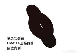
光谱学是测量紫外、可见、近红外和红外波段光强度的技术。光谱测量被广泛应用于多种领域,如颜色测量、化学成份的浓度测量或辐射度学分析、膜厚测量、气体成分分析等领域。在上世纪九十年代以来,微电子领域中的多象元光学探测器(例如CCD,光电二极管阵列)制造技术迅猛发展,使生产低成本扫描仪和CCD相机成为可能。美国海洋光学公司的微型光纤光谱仪使用了同样的CCD(CCD光谱仪)和光电二极管阵列探测器,可以对整个光谱进行快速扫描,不需要转动光栅。 海洋光学的微型光纤光谱仪通常采用光纤作为信号耦合器件,将被测光耦合到光谱仪中进行光谱分析。由于光纤的方便性,用户可以非常灵活的搭建光谱采集系统。其优势在于测量系统的模块化和灵活性,且测量速度非常快,可以用于在线分析。而且由于采用了低成本的通用探测器,降低了光谱仪的成本,从而也降低了整个测量系统的造价。 微型光纤光谱仪基本配置包括包括一个光栅,一个狭缝和一个探测器。这些部件的参数在选购光谱仪时必须详细说明。光谱仪的性能取决于这些部件的精确组合与校准,校准后光纤光谱仪,原则上这些配件都不能有任何的变动。海洋光学拥有广泛的光谱仪配置选择,使其性能最大化以满足客户要求。如果这些配置不符合您的要求,我们可以根据您的要求为您量身定做。 海洋光学微型光纤光谱仪选型① 光学分辨率光学分辨率是配置微型光纤光谱仪时经常被考虑的主要因素之一。当用户为了追求微型光纤光谱仪的高分辨率时,在选型时会选择具有尽可能多像元数探测器的微型光谱仪。而实际上光学分辨率不仅仅由探测器的像元数决定,还与狭缝宽度和光栅的刻线密度有关。所以当讨论分辨率时,通常用色散或用波长范围除以像元数。半高全宽值(FWHM),即最大峰值光强一半处所对应的谱线宽度是一种表述分辨率更好的方法(见上图)。用FWHM可以对不同光谱仪的实际光学性能进行直接对比。用这种表示方法可以避免一些缺陷,例如:有的光栅并没有用到全部像元;采用交叉式Czerny-Turner光路设计的光谱仪中,光学系统不能把狭缝清晰地成像在探测器上,这是由于光路中过大的反射角和固有的系统放大倍率造成的。http://ng1.17img.cn/bbsfiles/images/2012/04/201204122045_360970_1855403_3.jpg② 灵敏度灵敏度是配置光谱仪时所需要考虑的另一个因素。现在的主流微型光纤光谱仪都采用线阵探测器,所以灵敏度跟像素数没有任何关系。但面阵探测器例外,因为面阵探测器在垂直方向的每个像素都会被累积,在某种意义上垂直方向上的所有像素的累积可以被看成一个更大的像素。因此,在考虑某种应用对灵敏度的要求时,更重要的是看探测器的响应曲线。下图中给出了海洋光学微型光纤光谱仪采用的两种典型探测器的灵敏度响应曲线。http://ng1.17img.cn/bbsfiles/images/2012/04/201204122046_360971_1855403_3.jpg③ 信噪比信噪比也是选配微型光纤光谱仪的一个因素。对于CCD光谱仪,较高的灵敏度导致了较低的信噪比。在一定范围内,可以通过对光谱进行多次平均来提高信噪比。平均次数的平方根恰好是信噪比提高的倍数。例如,光谱平均100次,信噪比能提高10倍。有些应用需要较高的信噪比,此时用户应当比较在光谱仪中的光学平台和探测器的综合信噪比。需要强调的是,用户一定要搞清楚厂家给出的信噪比是不是整个光谱仪系统的信噪比,因为只有整个光谱仪系统的信噪比才是最重要的。一个信噪比高的探测器配一个性能不高的光路,那么它的高信噪比就没有实际意义。比较不同探测器和微型光纤光谱仪间的信噪比的比较好的方法是:测量100次,然后对每个像元计算平均值和标准偏差,信噪比等于平均值除以标准偏差。测量信噪比时,信号强度应当接近饱和,并设置正确的平滑值(如果需要的话)。④ 光栅选择光栅选择是最比较复杂的。通常有两个因素决定了光栅的选择:波长范围和光学分辨率。波长范围受限于所选择的探测器或光栅,或二者都有。光学分辨率不仅受限于光栅,还受限于狭缝宽度和探测器的像元数和像元尺寸。还要考虑第三个因素,即光栅还会影响系统的灵敏度,这是因为不同的光栅的闪耀波长(即最高效率)位置各不相同。当对系统进行最优化配置时,最好查看一下光栅的效率曲线。下图中是海洋光学微型光纤光谱仪采用的几种典型的600线/mm光栅的效率曲线,效率最高点从紫外区到近红外区。http://ng1.17img.cn/bbsfiles/images/2012/04/201204122047_360972_1855403_3.jpg⑤ 狭缝狭缝了也是选配微型光纤光谱仪的一个因素。微型光纤光谱仪有多种狭缝尺寸供您选择,狭缝安装在光纤接头处(见图),并且被永久的固定在光谱仪上。有两点需要记住,狭缝越小,光学分辨率越高;狭缝越大,进入光学平台的光通量越多,即灵敏度越高。从本质上说,需要折中兼顾光谱仪的分辨率和灵敏度。http://ng1.17img.cn/bbsfiles/images/2012/04/201204122047_360973_1855403_3.jpg⑥ 其他 选择微型光纤光谱仪的其他选项会相对容易一些。例如可以选择升级UV4探测器后,探测器上的标准BK7窗片将会被石英窗片替代,用来增强海洋光学微型光纤光谱仪在波长340nm以下紫外区的响应能力。而其它探测器,比如薄型背照式CCD或CMOS则不需要这个选项。而为了避免二、三级衍射效应的影响,可以通过在位于狭缝与消包层模式孔之间的SMA905连接器中安装长通滤光片或在探测器的窗口处安装OFLV消除高阶衍射滤光片。正如上面介绍的几个因素所表明的,通过一些简单的步骤就就可以配置好满足您应用的微型光纤光谱仪。除了光谱仪,我们可能还需要考虑种类纷杂的光源和采样附件。所以不必犹豫尽管向我们咨询有关仪器的一切问题,我们将会给您一套最适合您应用的微型光纤光谱仪配置。
在直读光谱仪的实际应用中,如C、P、S、As等元素的最优光谱线均在真空紫外波段,而空气中的氧气及水蒸气等会对这些谱线产生强烈的吸收,使光谱强度急剧减弱,影响元素测量,所以应当将光室中的空气除去。 目前主流市场上主要有两种方式可以实现真空紫外波段元素的测量,光室抽真空或充惰性气体(如氩气、氦气等)。 抽真空型的直读光谱仪需要用额外的真空泵,存在油蒸汽污染严重、噪音大等环境问题。同时,功耗高、真空稳定速度慢,仪器需长期开机,浪费严重。 光室充惰性气体能实现真空紫外探测能力的同时,还具有稳定时间短,无噪音等优点,且能避免由于真空系统造成的光室变形、仪器漂移和环境污染等问题,目前,市场主流光谱仪多采用CCD传感器作为检测装置,光室体积可做到很小,更有利于惰性气体环境建立,从而得到更好的紫外元素分析效果,且该项技术已经过十多年市场验证,稳定可靠。
各位高工!光谱仪的波段范围 190-500nm是什么意思啊!它起什么作用,要怎么选择啊!!!
现在做实验,老板让我查一下以下气体在可见光波段的吸收谱,二氧化碳,二氧化硫,臭氧,甲烷等。我在网上找了狠多,都没有发现结果,那位大哥帮帮忙给弄一下啊,谢谢了另外,那个附图是我用NIST MS Search查到的光谱图,但是横坐标为什么没有光谱单位呢??
做[url=https://insevent.instrument.com.cn/t/1p][color=#3333ff]近红外光谱[/color][/url]霉变检测,运用特征提取方法获取了一些波段,如1172nm,1902nm等,看文献中都有对波段的分析,比如该波段是由哪个基团的什么运动引起的,对应于什么物质(碳水化合物,水分,油),想请教下这些东西是怎么分析出来的,或者有大牛能否帮忙分析下我的特征波段,万分感谢!
[align=center][img]https://img1.17img.cn/17img/images/202404/uepic/c76fabfd-be4f-4b7f-9ef3-3be47874e493.jpg[/img][/align][align=center][color=#7f7f7f]4月2日,国仪量子研发人员正在操作W波段脉冲式电子顺磁共振波谱仪[/color][/align][color=#000000]“W波段脉冲式电子顺磁共振波谱仪的研制成功,使国仪量子成为目前国内能研制生产该类高端科学仪器的厂商。也标志着中国成为继德国之后,第二个有能力研发该型电子顺磁共振波谱仪的国家。”4月2日,国仪量子技术(合肥)股份有限公司传感事业部副总经理石致富站在最新研发的仪器前向记者介绍。[/color][color=#000000]根据揭榜项目任务书的项目目标和考核指标,国仪量子最终任务全部完成,部分指标超额完成。专家组召开验收会议,认为该产品达到了国际先进水平,此攻关任务已经完成。[/color][color=#000000]近年来,安徽在量子信息领域“从0到1”的原始创新不断突破:[/color][color=#000000]目前,安徽集聚量子科技产业链企业60余家、数量居全国首位,全国首条量子芯片生产线建成运行,全国首个量子信息未来产业科技园挂牌运营,量子专利授权量全国领先,以国盾量子、国仪量子、本源量子、问天量子、中电信量子集团等为龙头的量子高新技术企业不断涌现。[/color][color=#000000]安徽发展量子信息等未来产业,具有强劲的科技创新策源能力。[/color][color=#000000]国仪量子在2021年承接了安徽省制造业重点领域产学研用补短板产品和关键共性技术攻关任务,项目针对“W波段电子顺磁共振波谱仪”进行工程化、产品化开发,解决产品化实现涉及到的核心技术难题,研制出用户友好、皮实可靠,可产品化出售的W波段电子顺磁共振波谱仪。W波段电子顺磁共振波谱仪具有高分辨率、高灵敏度的优势,是一种重要的高端科学分析装置,将给生物、化学、物理以及交叉学科等领域提供一项强有力的研究手段,可用于进行蛋白质、RNA、DNA 的结构解析,从而解决生物学、医学、制药学中的关键问题。[/color][color=#000000]得益于中国科学技术大学、合肥国家实验室等高校与科研机构,合肥在量子信息技术的科研领域具有先发优势,为量子科技发展提供了强有力的人才和智力支撑。[/color][color=#000000]“我们团队在量子精密测量领域有着十多年的研究积累,以长相干、多比特、高精度量子操控为核心目标,目前已掌握了世界领先的高保真量子态调控技术、高灵敏度磁探测技术、微波收发技术、高精度扫描钻石探针技术等核心技术。”石致富说。[/color][color=#000000]“揭榜挂帅”是用市场竞争来激发创新活力的一种机制。国仪量子相关负责人表示,“揭榜挂帅”有助于选拔领头羊、先锋队,聚力突破关键共性技术瓶颈,提高制造业自主创新能力,带动产业链上下游的技术进步,强化供应链保障。[/color][color=#000000]未来,国仪量子将持续加强研发投入力度,在核心技术上不断追求更高标准。与用户协同创新,推动技术落地,赋能多个行业的升级发展,在全球量子领域逐渐发出中国声音,也让“安徽身影”更加活跃。[/color][来源:安徽经济网][align=right][/align]
想测试一个UV光源的波段是多少,需要用什么仪器?
BLL9G1214L-600 BLL9G1214LS-600[b]选型:[img=image.png]https://www.ldteq.com/public/ueditor/upload/image/20231121/1700537083899742.png[/img]LDMOS L波段雷达功率晶体管[/b]600 W LDMOS功率晶体管,适用于1.2 GHz至1.4 GHz频率范围内的L波段雷达应用[img=image.png]https://www.ldteq.com/public/ueditor/upload/image/20231121/1700537071420795.png[/img][b]特点和优势[/b]高效率出色的坚固性专为 L 波段操作而设计优异的热稳定性轻松控制电源集成双面ESD保护,实现出色的关断状态隔离脉冲格式灵活性高内部匹配,易于使用符合关于有害物质限制 (RoHS) 的指令 2002/95/EC[b]应用[/b]频率范围为 1.2 GHz 至 1.4 GHz 的 L 波段雷达应用[font=微软雅黑, &][size=15px][color=#333333] 立维创展ldteq.com专业代理Ampleon产品,拥有价格优势,欢迎咨询。[/color][/size][/font]
请教各位朋友:仪器:UV-3600+积分球1:我们测过自己的样品固体材料(200-3300Nm),发现在近红外区谱线震荡非常厉害,不成峰型。是否是因为红外区有空气水分子干扰?需要充氮气循环?2:确实小虫知识不足,我想请教UV-VIS-NIR+积分球主要测试材料漫反射的作用是什么呢? 是不是检测A-H基团的?3.问个初级问题,人体发出的红外波段大概是哪个范围呢?
请教各位朋友:仪器:UV-3600+积分球 1:我们测过自己的样品固体材料(200-3300Nm),发现在近红外区谱线震荡非常厉害,不成峰型。是否是因为红外区有空气水分子干扰?需要充氮气循环?2:确实小虫知识不足,我想请教UV-VIS-NIR+积分球主要测试材料漫反射的作用是什么呢? 是不是检测A-H基团的?3.问个初级问题,人体发出的红外波段大概是哪个范围呢?
请问,在NIR中,全波段翻译成英语的地道说法应该怎么翻译:有道翻译结果:full-wave bandall bandfull range感觉不太准确和专业
室外微波单稳探测器,探测范围61米。XX型户外微波单稳探测器提供可靠的三维户外探测。灵敏、场可调的探测回路能探测61米范围内走动、奔跑及爬越的入侵者。射程定点回路(RCO)专利技术,可以摒弃所有预定射程外的微波目标,这一独特的功能使380型排除来自定点回路外目标报警干扰,即使是非常大的微波目标如双轮拖车、树、火车、卡车或高架通道。XX型工作在K波段,天生对来自机场着陆系统,振动电缆航空雷达及其它微波入侵探测器的干扰不敏感。因为它的K波段频率是X波段的2.5倍,由入侵者产生的多路信号也是X波段的2.5倍,因此对缓慢移动入侵者的探测效果更好。XX型应用了零射程抑制回路(ZRS)专利技术,这种回路可显著减少由于风、雨、摆动和鸟产生的误报。无论是RCO还是ZRS都不会影响对探测区域内人类闯入者的探测。内置多路复用系统允许380型与其他西南微波收发器和对射系统紧邻而不会相互干扰。多路复用操作通过一个同步线缆(双绞线)联到每个传感器上。任意一个传感器或外部时钟设置为“主机”,而其它所有传感器则设置为“从机”。最多为16个传感器的一组探测器中,只能有一个探测器在指定时间工作。XX型可很容易完成设置或调节。振动电缆将探测器对准要保护的区域,加电并用几分钟建立探测区域的反射信号参考水平。选择从15至61米的预期RCO距离,进行走动测试以确定最佳灵敏控制设置。XX型通过带位置锁定的可旋转支架安装在任何坚固表面。各方向均为20º可调,还可安装在直径8.9-10.2厘米的圆柱上。还可与西南微波的对射探测器一起探测450米范围内的三维空间。
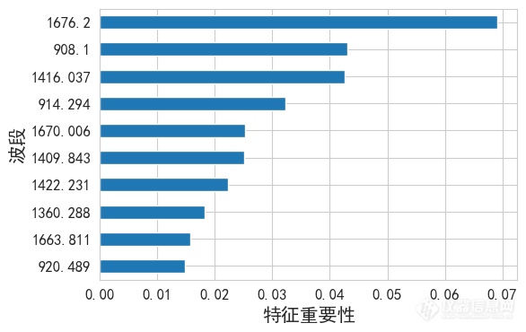
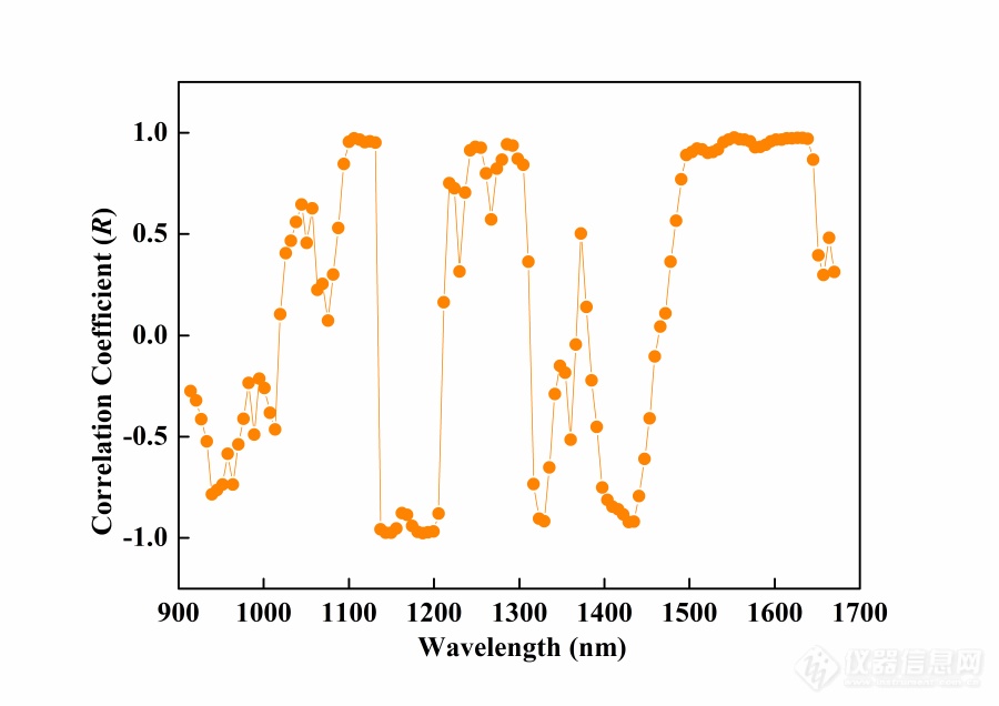
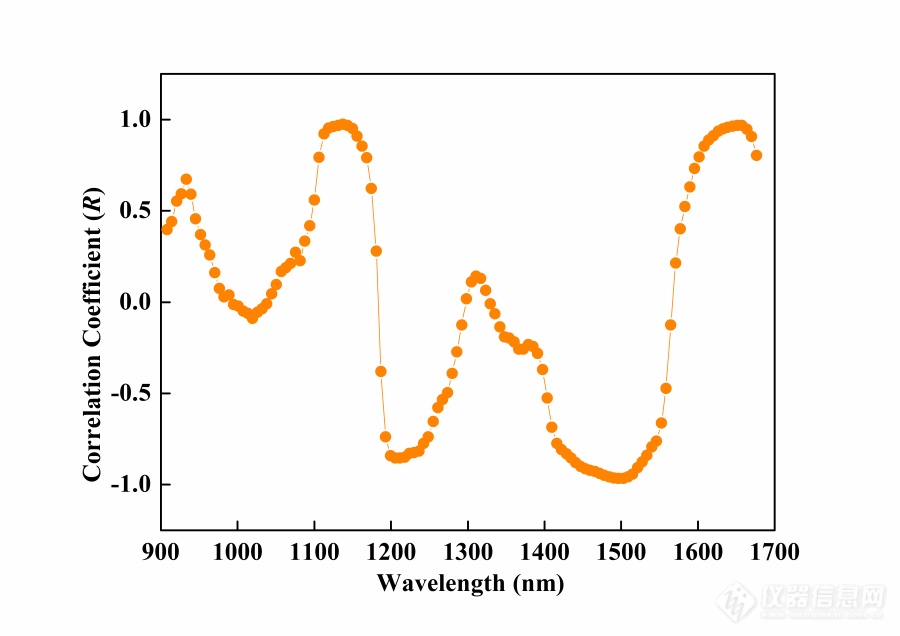
[font='times new roman'][size=16px][b]几种[/b][/size][/font][font='times new roman'][size=16px][b]波段选择[/b][/size][/font][font='times new roman'][size=16px][b]方法原理及应用[/b][/size][/font][size=14px][url=https://insevent.instrument.com.cn/t/1p][color=#3333ff]近红外光谱[/color][/url]数据的波段数有[/size][size=14px]多[/size][size=14px]个,特征维度较多,数据量较大,不同波段之间的信息冗余度高,具有一定的重叠性。本实验所用的试验样品是由多个成分组成的混合物,这样采集的[url=https://insevent.instrument.com.cn/t/1p][color=#3333ff]近红外光谱[/color][/url]就会由于没有混合均匀等原因常常掺杂着一些对非目标组分的吸收,导致光谱数据中的某些波段与样品的性质之间是比较差的关联关系,甚至是有一些关联关系是错误的,这就容易出现部分波段信息冗余的现象。同时,也会有其他一些因素对[url=https://insevent.instrument.com.cn/t/1p][color=#3333ff]近红外光谱[/color][/url]的准确性产生不利影响。[/size][size=14px]因此,为了得到更加有利于建立模型的[url=https://insevent.instrument.com.cn/t/1p][color=#3333ff]近红外光谱[/color][/url]数据,需要对一些无用的噪声波段进行剔除,找出那些含有较高信息量、容易分离、彼此相关度较低的波段,这就需要对[url=https://insevent.instrument.com.cn/t/1p][color=#3333ff]近红外光谱[/color][/url]进行波段选择。通过波段选择从原始[url=https://insevent.instrument.com.cn/t/1p][color=#3333ff]近红外光谱[/color][/url]中选择包含大量有效信息的波段子集,这些波段在建模中起主要作用,这样不但可以大大降低[url=https://insevent.instrument.com.cn/t/1p][color=#3333ff]近红外光谱[/color][/url]的维度,提高模型建立的速度,而且可以将光谱中存在的噪声信息剔除掉,只保留对提升模型准确性有利的信息。本文使用的波段选择方法使皮尔森相关系数法和随机森林法。[/size][font='times new roman'][size=16px][b]皮尔森相关系数法[/b][/size][/font][size=14px]相关系数法[/size][font='times new roman'][size=14px][54][/size][/font][size=14px]是将采集光谱的所有波段与颗粒的实际水分含量进行相关性计算,得到光谱每个波段与水分含量的相关系数。确定一定的阈值,将波段按照相关系数绝对值的大小进行排序,相关系数的绝对值超过阈值大小的波段保留下来,用这部分波段进行建模。[/size][size=14px]两个变量之间相关系数的大小在[/size][size=14px]-1~1[/size][size=14px]之间变化,当其中一个变量增大而另一个变量减小时,说明两个变量是负相关的,其相关系数为负数,并且相关系数越小,说明两个变量的负相关性越大;当其中一个变量增大,另一个变量也随之增大时,说明两个变量是正相关的,相关系数为正数,并且相关系数越大,说明两个变量间的正相关性越大。为了了解两个变量间的相关程度,以相关系数的绝对值[/size][size=14px]|R|[/size][size=14px]为标准判断两个变量的线性相关性大小,如下表所示。[/size][align=center][font='times new roman'][size=16px]表两个变量的相关性大小[/size][/font][/align][table][tr][td][align=center][font='times new roman'][size=16px]相关系数绝对值[/size][/font][font='times new roman'][size=16px]|R|[/size][/font][/align][/td][td][align=center][font='times new roman'][size=16px]相关性程度[/size][/font][/align][/td][/tr][tr][td][align=center][font='times new roman'][size=16px]≥[/size][/font][font='times new roman'][size=16px]0.95[/size][/font][/align][/td][td][align=center][size=13px]显著性相关[/size][/align][/td][/tr][tr][td][align=center][font='times new roman'][size=16px]≥[/size][/font][font='times new roman'][size=16px]0.8[/size][/font][/align][/td][td][align=center][size=13px]高度相关[/size][/align][/td][/tr][tr][td][align=center][size=13px]0.5[/size][font='宋体'][size=13px]≤|[/size][/font][font='宋体'][size=13px]R[/size][/font][size=13px]|0.35[/size][/font][font='times new roman'][size=16px]光谱波段[/size][/font][/align][size=14px] [/size][size=14px] [/size][size=14px]图中,绿色方格线覆盖的波段为相关系数绝对值[/size][size=14px]|R|[/size][size=14px]0.35[/size][size=14px]的波段。图中可以看出,与水分相关系数比较高的地方都在波段[/size][size=14px]908.1nm~1400nm[/size][size=14px]之间,将全光谱的[/size][size=14px]125[/size][size=14px]个波段降低到了[/size][size=14px]80[/size][size=14px]个。[/size][font='times new roman'][size=16px][b] [/b][/size][/font][font='times new roman'][size=16px][b]随机森林法[/b][/size][/font][size=14px]随机森林[/size][font='times new roman'][size=14px][55][/size][/font][size=14px]是一种并行的[/size][size=14px]bagging[/size][font='times new roman'][size=14px][56][/size][/font][size=14px]集成学习算法。随机森林使用的数据采集方法为“自助采样法”,自主采样法在数据集较小的情况下会有较好的训练结果。从一个包含[/size][size=14px][i]n[/i][/size][size=14px]个[/size][size=14px]样本的数据集[/size][size=14px][i]M[/i][/size][size=14px]中每次随机取出一个样本,对样本进行记录后把该样本重新放回[/size][size=14px][i]M[/i][/size][size=14px]中再进行随机取样,即有放回的随机取样,这样取出来的所有样本组成数据集[/size][size=14px][i]D[/i][/size][size=14px]。重复采样[/size][size=14px][i]n[/i][/size][size=14px]次,[/size][size=14px][i]M[/i][/size][size=14px]中有一部分数据在[/size][size=14px][i]D[/i][/size][size=14px]中重复出现多次,有一部分数据从来没有在[/size][size=14px][i]D[/i][/size][size=14px]中出现过,一个样本被取到的概率为[/size][size=14px]1/[/size][size=14px][i]n[/i][/size][size=14px],那么在[/size][size=14px][i]n[/i][/size][size=14px]次采样过程中样本一直不被取到的概率为([/size][size=14px]1-1/[/size][size=14px][i]n[/i][/size][size=14px])[/size][font='times new roman'][size=14px]1/[/size][/font][font='times new roman'][size=14px][i]n[/i][/size][/font][size=14px],通过求极限可以得到[/size][align=right][size=14px] [/size][size=14px] [/size][/align][size=14px]以采集的样本[/size][size=14px][i]D[/i][/size][size=14px]作为训练集,以未采集的样本数据集[/size][size=14px][i]P[/i][/size][size=14px]作为测试集。对数据集[/size][size=14px][i]D[/i][/size][size=14px]进行训练,并在训练过程中加入随机属性选择,这样就得到了一个决策树算法的[/size][size=14px]基学习器[/size][size=14px],然后把所有的[/size][size=14px]基学习器[/size][size=14px]组合起来,得到输出结果。在分类任务中,对每个[/size][size=14px]基学习器[/size][size=14px]对预测结果进行投票得到输出结果;在回归任务中,将每个[/size][size=14px]基学习器[/size][size=14px]的预测结果进行简单平均,求得的平均数作为最终的结果。[url=https://insevent.instrument.com.cn/t/1p][color=#3333ff]近红外光谱[/color][/url]水分预测是一个回归任务,因此选择随机森林回归法,[/size][size=14px]基学习器[/size][size=14px]的决策树为回归树,训练样本过将多个[/size][size=14px]基学习器回归[/size][size=14px]树进行训练,使用简单平均法获得预测结果,获得比单一回归树模型具有更高的预测准确率[/size][font='times new roman'][size=14px][57][/size][/font][size=14px]。随机森林回归的示意图如下图所示。[/size][align=center][font='times new roman'][size=16px]图[/size][/font][font='times new roman'][size=16px] [/size][/font][font='times new roman'][size=16px]随机森林回归示意图[/size][/font][/align][size=14px]随机森林回归算法中使用的基模型为[/size][size=14px]CART[/size][size=14px]回归树[/size][font='times new roman'][size=14px][58][/size][/font][size=14px],特征空间的划分和每个单元的输出值由这些回归树来决定。在回归树中,选择最佳的划分点需要对每个特征的所有值进行遍历,直到取得某个特征的某个值,使得损失函数最小,这就是最佳的划分点。假设有[/size][size=14px][i]n[/i][/size][size=14px]个[/size][size=14px]特征,每个特征有[/size][size=14px]个[/size][size=14px]取值,将特征空间划分为[/size][size=14px][i]M[/i][/size][size=14px]个[/size][size=14px]单元[/size][size=14px],[/size][size=14px]为[/size][size=14px]上输入[/size][size=14px]对应[/size][size=14px]的平均值,[/size][size=14px]则该过程的公式如下:[/size][align=right][size=14px] [/size][size=14px] [/size][/align][size=14px]选择最佳的划分点后,回归树的方程为:[/size][align=right][size=14px] [/size][size=14px] [/size][/align][size=14px]式中,[/size][size=14px][i]I([/i][/size][size=14px][i]x)[/i][/size][size=14px]为指示函数。[/size][size=14px]通过随机森林计算特征集中某一特征重要程度的过程如下:[/size][size=14px]([/size][size=14px]1[/size][size=14px])从数据集[/size][size=14px][i]M[/i][/size][size=14px]中通过随机自采样的方法获得数据集[/size][size=14px][i]D[/i][/size][size=14px],用数据集[/size][size=14px][i]D[/i][/size][size=14px]作为训练集进行建模,用没采集到的数据集[/size][size=14px][i]P[/i][/size][size=14px]进行验证,得到数据集[/size][size=14px][i]P[/i][/size][size=14px]的误差,记作[/size][size=14px][i]error[/i][/size][font='times new roman'][size=14px][i]1[/i][/size][/font][size=14px]。[/size][size=14px]([/size][size=14px]2[/size][size=14px])生成一组随机噪声数据,将随机噪声干扰数据加入到数据集[/size][size=14px][i]P[/i][/size][size=14px]的某一特征中,使得该特征对预测结果产生干扰,然后再次对数据集[/size][size=14px][i]P[/i][/size][size=14px]的误差进行计算,记作[/size][size=14px][i]error[/i][/size][font='times new roman'][size=14px][i]2[/i][/size][/font][size=14px]。[/size][size=14px]([/size][size=14px]3[/size][size=14px])计算[/size][size=14px][i]error[/i][/size][font='times new roman'][size=14px][i]2[/i][/size][/font][size=14px]与[/size][size=14px][i]error[/i][/size][font='times new roman'][size=14px][i]1[/i][/size][/font][size=14px]的差值。如果该特征是对预测结果起正向作用,则加入噪声数据后[/size][size=14px][i]error[/i][/size][font='times new roman'][size=14px][i]2[/i][/size][/font][size=14px]与[/size][size=14px][i]error[/i][/size][font='times new roman'][size=14px][i]1[/i][/size][/font][size=14px]的差值一定大于[/size][size=14px]0[/size][size=14px],反之则小于零。差值与这个特征对该模型预测精度的影响程度成正比。[/size][size=14px]([/size][size=14px]4[/size][size=14px])如果随机森林中有[/size][size=14px][i]N[/i][/size][size=14px]棵树,计算[/size][size=14px][i]N[/i][/size][size=14px]棵树对该特征[/size][size=14px][i]error2[/i][/size][size=14px]与[/size][size=14px][i]error1[/i][/size][size=14px]的差值的平均值,即[/size][align=right][size=14px] [/size][size=14px] [/size][/align][size=14px]([/size][size=14px]5[/size][size=14px])遍历数据集[/size][size=14px][i]P[/i][/size][size=14px]中的所有特征,求出每个特征的重要性。[/size][size=14px]用随机森林回归法对光谱数据与水分含量进行建模,得到数据[/size][size=14px]中特征[/size][size=14px]重要性排名,其中排名前十的特征如图[/size][size=14px]3-9[/size][size=14px]所示。[/size][align=center][img]https://ng1.17img.cn/bbsfiles/images/2020/09/202009031753099412_7932_3890113_3.png[/img][/align][align=center][font='times new roman'][size=16px]图[/size][/font][font='times new roman'][size=16px] [/size][/font][font='times new roman'][size=16px]随机森林特征选择排名前十的特征[/size][/font][/align][size=14px]特征重要性值的数据分布如下表所示。[/size][align=center][font='times new roman'][size=16px]表[/size][/font][font='times new roman'][size=16px] [/size][/font][font='times new roman'][size=16px]随机森林特征重要性分布[/size][/font][/align][table][tr][td][align=center][font='times new roman'][size=16px]数值分布[/size][/font][/align][/td][td][align=center][font='times new roman'][size=16px]特征重要性[/size][/font][/align][/td][/tr][tr][td][align=center][font='times new roman'][size=16px]最小值[/size][/font][/align][/td][td][align=center][font='times new roman'][size=16px]0.0022[/size][/font][/align][/td][/tr][tr][td][align=center][font='times new roman'][size=16px]1/4[/size][/font][font='times new roman'][size=16px]分位数[/size][/font][/align][/td][td][align=center][font='times new roman'][size=16px]0.0041[/size][/font][/align][/td][/tr][tr][td][align=center][font='times new roman'][size=16px]中位数[/size][/font][/align][/td][td][align=center][font='times new roman'][size=16px]0.0060[/size][/font][/align][/td][/tr][tr][td][align=center][font='times new roman'][size=16px]3/4[/size][/font][font='times new roman'][size=16px]分位数[/size][/font][/align][/td][td][align=center][font='times new roman'][size=16px]0.0081[/size][/font][/align][/td][/tr][tr][td][align=center][font='times new roman'][size=16px]最大值[/size][/font][/align][/td][td][align=center][font='times new roman'][size=16px]0.0692[/size][/font][/align][/td][/tr][tr][td][align=center][font='times new roman'][size=16px]平均值[/size][/font][/align][/td][td][align=center][font='times new roman'][size=16px]0.0080[/size][/font][/align][/td][/tr][/table][size=14px]分别以随机森林特征重要性数值分布的[/size][size=14px]1/4[/size][size=14px]分位数、中位数、[/size][size=14px]3/4[/size][size=14px]分位数和平均值为选择标准,以大于这个标准的特征重要性组合成的特征波段进行[/size][size=14px]PLS[/size][size=14px]建模,选择最佳的波段组合。建模的结果如下表所示。[/size][align=center][font='times new roman'][size=16px]表[/size][/font][font='times new roman'][size=16px] [/size][/font][font='times new roman'][size=16px]不同特征重要性的波段模型评价[/size][/font][/align][table][tr][td][align=center][size=13px] [/size][size=13px] [/size][size=13px]评价参数[/size][/align][size=13px]特征重要性[/size][/td][td][align=center][size=13px]R[/size][size=13px]MSECV[/size][/align][/td][td][align=center][size=13px]R[/size][size=13px]MSEP[/size][/align][/td][td][align=center][size=14px]R[/size][font='times new roman'][size=14px]p[/size][/font][/align][/td][/tr][tr][td][align=center][size=13px]全波段[/size][/align][/td][td][align=center][size=13px]0.242[/size][/align][/td][td][align=center][size=13px]0.221[/size][/align][/td][td][align=center][size=13px]0[/size][size=13px].9[/size][size=13px]60[/size][/align][/td][/tr][tr][td][align=center][size=13px]0.0041[/size][/align][/td][td][align=center][size=13px]0.222[/size][/align][/td][td][align=center][size=13px]0.214[/size][/align][/td][td][align=center][size=13px]0[/size][size=13px].9[/size][size=13px]80[/size][/align][/td][/tr][tr][td][align=center][size=13px]0.0060[/size][/align][/td][td][align=center][size=13px]0.216[/size][/align][/td][td][align=center][size=13px]0.209[/size][/align][/td][td][align=center][size=13px]0[/size][size=13px].[/size][size=13px]983[/size][/align][/td][/tr][tr][td][align=center][size=13px]0.0080[/size][/align][/td][td][align=center][size=13px]0.228[/size][/align][/td][td][align=center][size=13px]0.225[/size][/align][/td][td][align=center][size=13px]0[/size][size=13px].9[/size][size=13px]75[/size][/align][/td][/tr][tr][td][align=center][size=13px]0.0081[/size][/align][/td][td][align=center][size=13px]0.2[/size][size=13px]3[/size][size=13px]2[/size][/align][/td][td][align=center][size=13px]0.230[/size][/align][/td][td][align=center][size=13px]0[/size][size=13px].9[/size][size=13px]6[/size][/align][/td][/tr][/table][size=14px]很明显,通过随机森林方法计算出各个特征的重要性,以[/size][size=14px]0.0060[/size][size=14px]作为最低标准选择的波段用来建立[/size][size=14px]PLS[/size][size=14px]模型的效果最好。选择的波段如下图所示。[/size][align=center][font='times new roman'][size=16px]图[/size][/font][font='times new roman'][size=16px] [/size][/font][font='times new roman'][size=16px]随机森林波段选择[/size][/font][/align][size=14px] [/size][size=14px] [/size][size=14px]图中绿色背景的是通过随机森林选择的[url=https://insevent.instrument.com.cn/t/1p][color=#3333ff]近红外光谱[/color][/url]波段,其波段主要分布在[/size][size=14px]908.1nm~1150nm[/size][size=14px]和[/size][size=14px]1350nm~1500nm[/size][size=14px]之间,将[/size][size=14px]125[/size][size=14px]个光谱波段降低到了[/size][size=14px]60[/size][size=14px]个,[/size][size=14px]降维效果[/size][size=14px]和模型评价效果均优于相关系数法。因此在流化床制粒过程[url=https://insevent.instrument.com.cn/t/1p][color=#3333ff]近红外光谱[/color][/url]的建模中应用随机森林法进行波段选择。[/size]
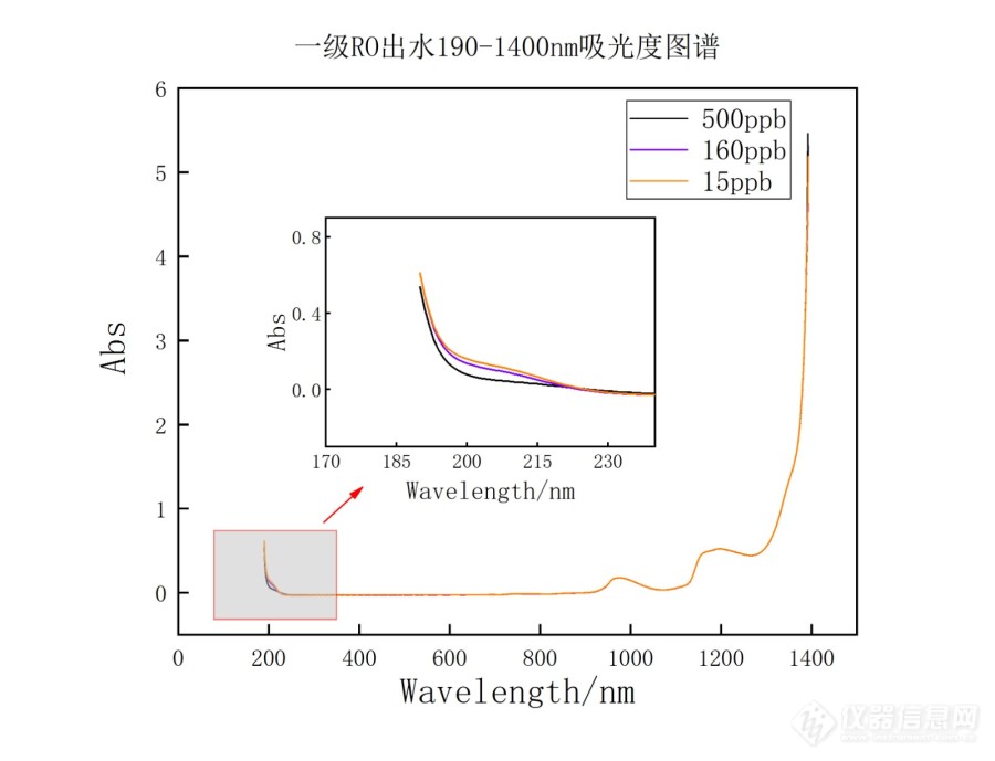
[size=24px]电子级水/超纯水 远紫外波段吸光度检测[/size]请教各位大神,对于类似超纯水、半导体行业用水这种水质指标极高的水,远紫外波段(<200nm)吸光度应该如何检测?有几个疑问,请论坛大神解答;1.远紫外波段真空紫外光易被空气吸收,且光程短,如何适配比色皿,排除空气干扰?2.类似安捷伦、lambda这些仪器为什么标称170nm-3300nm都可以检测,但是实际应用中最低只能检测到190nm处?3.为获得特定波长处(如185nm,超纯水TOC降解波段)吸光度,该如何实现?[img=,690,528]https://ng1.17img.cn/bbsfiles/images/2023/03/202303291111198785_2326_5961157_3.jpg!w690x528.jpg[/img]
紫外线传感器是传感器的一种,可以利用光敏元件通过光伏模式和光导模式将紫外线信号转换为可测量的电信号,目前紫外线传感器材料主要是GaN和SiC这两大类。GaN材质的传感器目前知名度比较高的是韩国Genicom的紫外线传感器,传感器的波段从200-510nm均有相对应的传感器来检测。针对UVA波段,主要有IIC、电流、电压输出方式的传感器。在智能穿戴以及一些要求传感器体积尽可能小或者对PCB尺寸要求比较小的场所可以使用GUVA-C32SM或者GUVA-S12SD(SMD3528封装)。针对一些要求温度稳定性比较高的场所,还有金属TO-46(GUVA-T11GD-L)、TO-39(GUVA-T21GD-U)、TO-5(GUVA-T21GH)封装产品。TO-5封装的产品里面都集成了运算放大电路,0-5V模拟量输出。方便使用。主要运用于UVA灯的检测,UV固化等。UVB传感器主要是用于检测B波段的LED灯、皮肤光疗仪以及UVI检测。UVI指数指标主要是针对B波段的紫外线而言的。主要运用到的型号有GUVB-C31SM(IIC输出)、GUVB-T11GD-L(电流输出)、GUVB-T21GH(0-5V输出)。UVC传感器由于具有日盲特性,除了用于紫外线消毒监测上,还可以用于火焰探测。火焰探测的前提条件是传感器能够检测极低辐射强度的紫外线,同时传感器的暗电流必须非常低,这样SiC材质的传感器就能满足需求目前知名度比较高的是德国Sglux的SiC紫外线传感器。该类型传感器能够耐高温以及强紫外线辐射。该厂商的传感器代表型号有SG01D,该传感器TO-5封装,带有聚光镜,在10uw/cm2辐射强度下可以输出350nA的电流。感光芯片面积可以从0.06mm2~36mm2。同时该产商TOCON-ABC系列可以在1.8pw/cm2~18w/cm2的范围内都有相对应的传感器来监测,能应对各种各样的需求。
黑碳监测仪BCA-I是基于光学衰减法的监测仪器,可连续实时监测大气中黑碳气溶胶的质量浓度。其工作原理是利用吸附在带状石英滤纸上的黑碳气溶胶在不同光学波段的吸收特性不同,实现对黑碳气溶胶的总量监测。它主要由光学系统、气体采样系统、走纸机构、数据采集与处理系统等组成。 仪器工作时,在抽气泵的驱动下,环境空气以恒定的流速连续地被抽入仪器的气体监测室,经滤纸过滤后,黑碳颗粒附着在透光均匀的石英纤维滤纸上。每隔一个时间周期,仪器开/关测量光源和参考光源一次,分别测量透过滤纸的气溶胶采样区和参考区的光强。根据光强信号,计算每个测量周期的采样区的光学衰减增量,得到该测量周期内收集的黑碳气溶胶质量,再除以这段时间的采样空气体积,即可以计算出采样空气流中的平均黑碳浓度。BCA-I的测量循环周期如下:(1) 打开光源,让系统稳定;(2) 测量光源照射时采样点和参考点的光强信号(SB和RB);(3) 测量仪器的空气流量F;(4) 测量仪器内的温度T;(5) 关闭光源;(6) 进行计算,显示数据,数据写入存储器,并通过串口发送至上位机;(7) 等待下一个测量周期(回到步骤(1))的开始。 当累积衰减量达到一定数值时,系统认为滤纸上黑碳颗粒沉积量已经达到一定数量,需要进行换纸以便继续测量,此时,系统将自动控制进纸电机进行进纸,再又转纸电机进行转纸。换纸期间,为了使气泵在不间断工作的情况下保持滤纸干净,系统控制气体从旁路进气口进入,经过三通电磁阀的旁路通道,最后通过排气口排除仪器外。 由于参考点的滤纸和其它光学器件的透光率在整个测量过程中不会发生变化,所以参考点的测量信号可以用来修正光源光强的微小变化,以提高仪器的准确性。合肥霍金光电生产的七波段黑碳气溶胶监测仪设计思路和技术路线新颖,各项性能指标均达到国际同类产品水平,并在局部功能设计上优于国外同类产品,总体技术处于国内领先水平。合肥霍金光电研发团队在合肥物质科学研究院环境光学中心“七波段碳黑气溶胶分析仪”技术基础理论研究的基础上,通过技术创新、“二次开发”,并依据中国气象局、中国环保局等用户的使用意见,完善了设计与工艺,在机械结构、软件功能、操控界面、数据存储格式及存储容量等方面,使之更符合国内客户的使用习惯,已完全具备了产业化实施的全部条件,首批生产的10台样机全部满足设计要求,与此同时,公司已获得针对检测方法和仪器设计的发明专利。[align=center] [b]表1 BCA7技术指标[/b][/align][table=607][tr][td=1,1,175][size=2]名 称[/size][/td][td=1,1,432][align=center][size=2]技术指标[/size][/align][/td][/tr][tr][td=1,1,175][size=2]测量范围[/size][/td][td=1,1,432][align=center][size=2]0 ng/m[sup]3[/sup]~1000,000ng/m[sup]3[/sup][/size][/align][/td][/tr][tr][td=1,1,175][align=center][size=2]测量精度[/size][/align][/td][td=1,1,432][align=center][size=2]5%[/size][/align][/td][/tr][tr][td=1,1,175][align=center][size=2]系统噪声[/size][/align][/td][td=1,1,432][align=center][size=2]≤100 ng/m[sup]3[/sup][/size][/align][/td][/tr][tr][td=1,1,175][size=2]光源波长[/size][/td][td=1,1,432][align=center][size=2]370nm,470nm,520nm,590nm,660nm,880nm,950nm[/size][/align][/td][/tr][tr][td=1,1,175][size=2]数字输入/输出[/size][/td][td=1,1,432][align=center][size=2]RS-232接口[/size][/align][/td][/tr][tr][td=1,1,175][size=2]仪器显示[/size][/td][td=1,1,432][align=center][size=2]8行液晶显示屏[/size][/align][/td][/tr][tr][td=1,1,175][size=2]采样流量[/size][/td][td=1,1,432][align=center][size=2]1~8升/分(内置泵,可调)[/size][/align][/td][/tr][tr][td=1,1,175][size=2]数据存储介质、容量[/size][/td][td=1,1,432][align=center][size=2](1)内部存储器、11天以上[/size][size=2](2)USB接口,一年以上(可选)[/size][/align][/td][/tr][tr][td=1,1,175][size=2]通信方式[/size][/td][td=1,1,432][align=center][size=2]GPS 通信(可选)[/size][/align][/td][/tr][tr][td=1,1,175][size=2]操作环境[/size][/td][td=1,1,432][align=center][size=2]-30~40℃,一般室内环境[/size][/align][/td][/tr][tr][td=1,1,175][size=2]电源[/size][/td][td=1,1,432][align=center][size=2]220V±22V,50Hz±1Hz[/size][/align][/td][/tr][tr][td=1,1,175][size=2]重量[/size][/td][td=1,1,432][align=center][size=2]21公斤[/size][/align][/td][/tr][tr][td=1,1,175][size=2]机箱尺寸[/size][/td][td=1,1,432][align=center][size=2]约440mm×260mm×320mm[/size][/align][/td][/tr][/table]
中国科技网讯 据物理学家组织网日前报道,美国能源部斯坦福直线加速器中心国家加速器实验室的研究人员,采用金刚石细薄片把直线加速器的相干光源转化为手术刀般更精确的工具,以探测纳米世界。改进后的激光脉冲可在X射线波长更窄频带高强度聚焦,开展以前所不能为的实验。该研究结果刊登在《自然·光子学》杂志上。 这个过程被称为“自激注入”,金刚石将激光束过滤为单一的X射线颜色,然后将其放大。研究人员可以在原子水平研究和操纵物质上有更强的能力,传送更为清晰的物质、分子和化学反应的影像。 人们谈论“自激注入”已经近15年,直到2010年斯坦福线性加速器中心成立时,才由欧洲自由电子激光器和德国电子加速器研究中心的研究人员提出,并由来自斯坦福线性加速器中心和阿贡国家实验室的工程队伍将其建立。“自激注入”可潜在地产生更高强度的X射线脉冲,显著高于目前直线加速器相干光源的性能。每个脉冲增加的强度可以用来深入探测复杂的材料,以帮助解答诸如高温超导体等特殊物质或拓扑绝缘体中复杂电子态等问题。 直线加速器相干光源通过接近光速的电子群加速激光束,用一系列磁体将其设定为“之”字路径。这将迫使电子发射X射线,聚集成亮度超过之前10亿倍的激光脉冲。如果没有“自激注入”,这些X射线激光脉冲包含的波长(或颜色)范围比较宽,无法被所有的实验使用。之前在直线加速器相干光源创造更窄波段(即更精确波段)的方法则会导致大量的强度损失。 研究人员在可产生X射线的130米长磁体的中间段安装了一片金刚石晶体,由此创建了一个精确的X射线波段,并且使直线加速器相干光源更像是“激光”。该中心物理学家黄志荣(音译)说:“如果我们完成系统的优化,并添加更多的波荡,所产生的脉冲集中的强度将达10倍之多。”目前世界各地的相关实验室已经趋之若鹜,计划将这一重要进展与自身的X射线激光设施相结合。(记者 华凌) 《科技日报》(2012-09-17 二版)
1 引言 微型光谱仪具体模块化和高速采集的特点,在系统集成和现场检测的场合得到了广泛的应用。结合光源、光纤、测量附件,可以搭配成各种光学测量系统。 光谱仪器是应用光学技术、电子技术及计算机技术对物质的成分及结构等进行分析和测量的基本设备,广泛应用于环境监测、工业控制、化学分析、食品品质检测、材料分析、临床检验、航空航天遥感及科学教育等领域。由于传统的光谱仪存在着结构复杂、使用环境受限、不便携带及价格昂贵等不足,不能满足现场检测和实时监控的需求。因此,微型光纤光谱仪成为光谱仪器发展的一个重要的研究方向。近年来,由于光纤技术、光栅技术及阵列式探测器技术的发展和成熟,使得光谱检测系统形成了光源、采样单元及摄谱单元相分离的结构形式,整个系统结构更具模块化,使用更加方便灵活,从而使微型光纤光谱仪成为现场检测和实时监控的首选仪器。 2 微型光谱仪结构 传统的光谱仪光学系统结构复杂,需通过旋转光栅对整个光谱进行扫描,测量速度慢,并且对某些样品还需经过特定的预处理,并要放在仪器的固定样品室内进行测量。与此相比,微型光纤光谱仪有很多优点,如:速度快、价格低、体积小、重量轻及全谱获取,而且通过光纤传导可以脱离样品室测量,适用于在线实时检测。 光谱仪微型化设计的实现得益于摄谱结构的优化。微型光纤光谱仪使用非对称交叉式Czerny-Turner分光结构,此光学结构的设计是在Czerny- Turner结构基础上进行光路的改进,使光谱仪内部构件布局更紧凑,可进一步小型化。摄谱结构光学平台的优化设计使微型光纤光谱仪内部无移动部件,光学元件都采用反射形式,可在一定程度上减少像差,并使工作光谱范围不受材料影响。微型光谱仪的固定化光学平台适合于震动及窄空间等复杂的工作环境。 3 微型光谱仪特点 光纤传导技术:光纤技术的发展,使待测物脱离了固定样品池的限制,采样方式变得更加灵活,适合于远距离样品品质监控。由于光纤对光信号的传输作用,使得光谱仪可以远离外界环境的干扰,保证光谱仪的长期可靠运行。 CCD阵列探测器技术:将经光栅分光后的作用光在探测器上同时瞬间采集,而不必移动光栅,因此样品光谱采集速度及快,并通过计算机实时输出。 光栅技术:全息光栅具有较小的杂散光,而机械刻划光栅具有更高的反射率和灵敏度。 计算机技术:电子计算技术的发展极大地提高了光谱仪的智能控制和处理能力。 4 微型光谱仪应用 随着微型光谱仪应用测量系统的不断拓展,其快速高效分析及便携式实时应用的优势逐渐显现出来,光谱分析技术正逐步从实验室分析走向现场实时检测。依据现阶段实际应用现状,微型光纤光谱仪在以下领域得到广泛的应用。 透射吸收测量:透射吸收测量用于测定液体或气体中介质对作用光的吸收,依据比耳定律,吸光度正比于摩尔吸收率、光程和样品介质浓度。 反射测量:反射测量方式分为镜面反射和漫反射测量,在实际测量中,可以采用不同的参考白板和测量角度来进行区分。反射测量用于测定样品的化学成分及表面颜色相关信息。 发光二极管(LED)测量:LED测量系统用于LED光源的绝对光谱强度及颜色指标测量。 激光测量:根据激光光谱的特征,检测系统配置高分辨率微型光纤光谱仪,同时可用积分球或余弦校正器来衰减入射光,以避免CCD探测器的饱和。 荧光测量:荧光测量因其光谱信号特别弱,因此需要一个高灵敏的探测器及一个高效率的滤光片,将样品激发出的微弱信号光和高强度的激发光区别开来。 氧含量测量:氧含量是通过光纤探头尖端荧光团的荧光强度的衰减来进行测量,应用荧光淬灭原理可以测量溶解氧或气态氧的分压,从而探测出环境的氧含量。 拉曼光谱测量:拉曼光谱与红外吸收光谱同为研究物质的分子振动能级从而分析物质的组成,但相对于红外吸收光谱,拉曼光谱的谱线较为简单且具有独特性,而且被测物不需进行前处理,因此在判断物质组成成分时有明显的优势。拉曼光谱测量系统特别适用于反应过程监控、产品识别、遥感及介质中高散射粒子的判定。 激光诱导击穿光谱(LIBS)测量:LIBS是一种用于固体、液体及气体中进行实时、定性及半定量的光谱元素分析技术,其工作原理是高强度的脉冲激光聚焦在样品表面,脉宽为10ns的激光脉冲蒸发样品产生等离子体,随着等离子体的冷却,处于激发态的原子发射出元素的特征光谱,这个光谱被光纤探头收集并传送到光谱仪,通过光谱分析软件中预存的样品特征光谱进行比对分析。 5 结论 微型光谱仪具有系统模块化和搭建灵活性的优势,因此在实际生产研究中,仅需配一套光谱仪,应用不同的测试附件就可以对各种不同的样品进行实时检测。同时,微型光纤光谱仪具有内部结构紧凑、无移动部件、波长范围宽、测量速度快、价格低的特点,在工业在线监控及便携式检测系统开发等领域提供了广阔的应用发展空间。(选自网络)
随着我国的仪器仪表工业的蓬勃发展,体积小巧、无油环保的微型真空泵、微型气泵、微型水泵得到越来越广泛的使用。如何才能在规格繁多的微型泵中选择最适合您的产品呢? 根据微型泵的用途,可以分为几类来讨论: 详见http://www.weichengkj.com/test-data/chose.htm
替代钴源辐照 无损伤 无残毒 低能耗 操作简便2013年07月11日 来源: 中国科技网 作者: 过国忠 陆文晓 中国科技网江苏无锡7月10日电 我国科研人员历时5年多,研制出国内首台L波段10MeV/40kW工业辐照电子加速器。今天,这项由无锡爱邦辐射技术有限公司、中国科学院高能物理研究所联合承担的重大科研成果,顺利通过专家鉴定。 据了解,大功率工业辐照电子直线加速器是一类适用于综合辐照加工的当代最先进的高技术设备。用电子加速器产生的高能电子束照射可使一些物质产生物理、化学和生物学效应,并能有效地杀灭病菌、病毒和害虫,可广泛应用于工业生产中的材料改性、新材料制作、环境保护、加工生产、医疗卫生用品灭菌消毒和食品灭菌保鲜等领域。它同钴源辐照一样,具有常温、无损伤、无残毒、环保、低能耗、运行操作简便、自动化程度高、适宜于大规模工业化生产等特点。“与钴源相比,其最大优点是辐照束流集中定向,能源利用充分,辐照效率高,不产生放射性废物,具有明显的社会经济效益和不可估量的潜在价值,是目前国际上备受关注的高科技领域之一。”无锡爱邦辐射技术有限公司总经理张祥华说。 据中国科学院高能物理研究所有关科研人员透露,开发L波段10MeV/40kW工业辐照电子加速器,涉及高气压、高电压、高真空、电子学、计算机、微波技术、电气控制技术、机械设计与加工、样品机械传输装置、辐射剂量学等多学科。从2008年开始,无锡爱邦辐射技术有限公司、中国科学院高能物理研究所联合组成攻关组,在三极电子枪、L波段聚束段加速结构、恒流充电式脉冲调制器、大功率水冷系统和大功率扫描系统等关键技术获得突破,成功研制出国内首台L波段10MeV/40kW工业辐照电子加速器。经国家有关部门检测显示,束流平均功率大于45kW,微波功率到束流功率的转换效率大于75%。(记者 过国忠 通讯员 陆文晓) 《科技日报》(2013-7-11 一版)
哪些波段的波属于噪声?
卫星监测定义:通过搭载在卫星上的观测仪器对大气、云和地表等变化的监测。草原和森林火灾的监测 草原或森林发生火灾的地区,温度远高于周围地区。采用3.7μm波段,对高温区特别敏感,利用3.7μm可以监测林区和草原发生的火灾。 http://www.kepu.net.cn/gb/earth/weather/observe/images/obs009_1801_pic.jpg红色部分表示内蒙古地区林区及草原火灾图象
[font='times new roman'][size=16px][b]波段选择[/b][/size][/font][font='times new roman'][size=16px][b]结合[/b][/size][/font][font='times new roman'][size=16px][b]模型转移[/b][/size][/font][font='times new roman'][size=16px][b]用于提高定量模型的预测能力[/b][/size][/font][font='times new roman'][size=16px]为了提高模型的准确性和[/size][/font][font='times new roman'][size=16px]稳定[/size][/font][font='times new roman'][size=16px]性,使用相关系数([/size][/font][font='times new roman'][size=16px]CC[/size][/font][font='times new roman'][size=16px])法、无信息变量消除算法([/size][/font][font='times new roman'][size=16px]UVE[/size][/font][font='times new roman'][size=16px])、[/size][/font][font='times new roman'][size=16px]VIP[/size][/font][font='times new roman'][size=16px]算法和吸光度[/size][/font][font='times new roman'][size=16px]-[/size][/font][font='times new roman'][size=16px]浓度变化率([/size][/font][font='times new roman'][size=16px]RATC[/size][/font][font='times new roman'][size=16px])进行波段选择。参数[/size][/font][font='times new roman'][size=16px]RMSECV[/size][/font][font='times new roman'][size=16px]用来评估[/size][/font][font='times new roman'][size=16px]PLS[/size][/font][font='times new roman'][size=16px]模型的预测能力。[/size][/font][font='times new roman'][size=16px]相关系数[/size][/font][font='times new roman'][size=16px]表为相关系数波段选择的结果,以每个变量点下光谱的吸光度值与一级数据的相关系数的绝对值作为结果考察的阈值。结果表明,当相关系数绝对值设置为[/size][/font][font='times new roman'][size=16px]0.9[/size][/font][font='times new roman'][size=16px]时,得到的模型结果最优。[/size][/font][font='times new roman'][size=16px][i]R[/i][/size][/font][font='times new roman'][size=16px]2[/size][/font][font='times new roman'][size=16px][i]c[/i][/size][/font][font='times new roman'][size=16px],[/size][/font][font='times new roman'][size=16px][i]R[/i][/size][/font][font='times new roman'][size=16px]2[/size][/font][font='times new roman'][size=16px][i]cv[/i][/size][/font][font='times new roman'][size=16px],[/size][/font][font='times new roman'][size=16px]RMSEC[/size][/font][font='times new roman'][size=16px]和[/size][/font][font='times new roman'][size=16px]RMSECV[/size][/font][font='times new roman'][size=16px]分别为[/size][/font][font='times new roman'][size=16px]0.965[/size][/font][font='times new roman'][size=16px],[/size][/font][font='times new roman'][size=16px]0.959[/size][/font][font='times new roman'][size=16px],[/size][/font][font='times new roman'][size=16px]2.0946[/size][/font][font='times new roman'][size=16px]和[/size][/font][font='times new roman'][size=16px]2.3404[/size][/font][font='times new roman'][size=16px]。图[/size][/font][font='times new roman'][size=16px] [/size][/font][font='times new roman'][size=16px](a)[/size][/font][font='times new roman'][size=16px]为[/size][/font][font='times new roman'][size=16px]|[/size][/font][font='times new roman'][size=16px][i]R[/i][/size][/font][font='times new roman'][size=16px]|[/size][/font][font='times new roman'][size=16px]阈值[/size][/font][font='times new roman'][size=16px]0.9[/size][/font][font='times new roman'][size=16px]时的相关系数图,图[/size][/font][font='times new roman'][size=16px] [/size][/font][font='times new roman'][size=16px](b)[/size][/font][font='times new roman'][size=16px]为根据图[/size][/font][font='times new roman'][size=16px](a)[/size][/font][font='times new roman'][size=16px]选出的用于建模的变量点,从图中可以看出,选出的变量点与图中的特征波段[/size][/font][font='times new roman'][size=16px]1100[/size][/font][font='times new roman'][size=16px] [/size][/font][font='times new roman'][size=16px]nm[/size][/font][font='times new roman'][size=16px], 1400[/size][/font][font='times new roman'][size=16px] [/size][/font][font='times new roman'][size=16px]nm, 1600[/size][/font][font='times new roman'][size=16px] [/size][/font][font='times new roman'][size=16px]nm[/size][/font][font='times new roman'][size=16px]相一致,模型结果有所提高。[/size][/font][align=center][font='times new roman']表[/font][font='times new roman']相关系数波段选择结果比较[/font][/align][table][tr][td][align=center][font='times new roman']|[/font][font='times new roman'][i]R[/i][/font][font='times new roman']|[/font][font='times new roman']阈值[/font][/align][/td][td][align=center][font='times new roman'][i]R[/i][/font][font='times new roman'][size=13px][i]2[/i][/size][/font][font='times new roman'][size=13px][i]c[/i][/size][/font][/align][/td][td][align=center][font='times new roman'][i]R[/i][/font][font='times new roman'][size=13px][i]2[/i][/size][/font][font='times new roman'][size=13px][i]cv[/i][/size][/font][/align][/td][td][align=center][font='times new roman']RMSEC[/font][/align][/td][td][align=center][font='times new roman']RMSECV[/font][/align][/td][td][align=center][font='times new roman']LVs[/font][/align][/td][td][align=center][font='times new roman']变量点数[/font][/align][/td][/tr][tr][td][align=center][font='times new roman']0.1[/font][/align][/td][td][align=center][font='times new roman']0.961[/font][/align][/td][td][align=center][font='times new roman']0.948[/font][/align][/td][td][align=center][font='times new roman']2.2121[/font][/align][/td][td][align=center][font='times new roman']2.5414[/font][/align][/td][td][align=center][font='times new roman']3[/font][/align][/td][td][align=center][font='times new roman']120[/font][/align][/td][/tr][tr][td][align=center][font='times new roman']0.2[/font][/align][/td][td][align=center][font='times new roman']0.961[/font][/align][/td][td][align=center][font='times new roman']0.952[/font][/align][/td][td][align=center][font='times new roman']2.2135[/font][/align][/td][td][align=center][font='times new roman']2.5229[/font][/align][/td][td][align=center][font='times new roman']3[/font][/align][/td][td][align=center][font='times new roman']113[/font][/align][/td][/tr][tr][td][align=center][font='times new roman']0.3[/font][/align][/td][td][align=center][font='times new roman']0.961[/font][/align][/td][td][align=center][font='times new roman']0.953[/font][/align][/td][td][align=center][font='times new roman']2.2162[/font][/align][/td][td][align=center][font='times new roman']2.489[/font][/align][/td][td][align=center][font='times new roman']3[/font][/align][/td][td][align=center][font='times new roman']104[/font][/align][/td][/tr][tr][td][align=center][font='times new roman']0.4[/font][/align][/td][td][align=center][font='times new roman']0.961[/font][/align][/td][td][align=center][font='times new roman']0.95[/font][/align][/td][td][align=center][font='times new roman']2.2118[/font][/align][/td][td][align=center][font='times new roman']2.5335[/font][/align][/td][td][align=center][font='times new roman']3[/font][/align][/td][td][align=center][font='times new roman']96[/font][/align][/td][/tr][tr][td][align=center][font='times new roman']0.5[/font][/align][/td][td][align=center][font='times new roman']0.961[/font][/align][/td][td][align=center][font='times new roman']0.954[/font][/align][/td][td][align=center][font='times new roman']2.1921[/font][/align][/td][td][align=center][font='times new roman']2.469[/font][/align][/td][td][align=center][font='times new roman']3[/font][/align][/td][td][align=center][font='times new roman']86[/font][/align][/td][/tr][tr][td][align=center][font='times new roman']0.6[/font][/align][/td][td][align=center][font='times new roman']0.963[/font][/align][/td][td][align=center][font='times new roman']0.951[/font][/align][/td][td][align=center][font='times new roman']2.1396[/font][/align][/td][td][align=center][font='times new roman']2.5285[/font][/align][/td][td][align=center][font='times new roman']3[/font][/align][/td][td][align=center][font='times new roman']77[/font][/align][/td][/tr][tr][td][align=center][font='times new roman']0.7[/font][/align][/td][td][align=center][font='times new roman']0.944[/font][/align][/td][td][align=center][font='times new roman']0.951[/font][/align][/td][td][align=center][font='times new roman']2.1345[/font][/align][/td][td][align=center][font='times new roman']2.4731[/font][/align][/td][td][align=center][font='times new roman']3[/font][/align][/td][td][align=center][font='times new roman']73[/font][/align][/td][/tr][tr][td][align=center][font='times new roman']0.8[/font][/align][/td][td][align=center][font='times new roman']0.964[/font][/align][/td][td][align=center][font='times new roman']0.955[/font][/align][/td][td][align=center][font='times new roman']2.1185[/font][/align][/td][td][align=center][font='times new roman']2.399[/font][/align][/td][td][align=center][font='times new roman']3[/font][/align][/td][td][align=center][font='times new roman']61[/font][/align][/td][/tr][tr][td][align=center][font='times new roman']0.9[/font][/align][/td][td][align=center][font='times new roman']0.965[/font][/align][/td][td][align=center][font='times new roman']0.959[/font][/align][/td][td][align=center][font='times new roman']2.0946[/font][/align][/td][td][align=center][font='times new roman']2.3404[/font][/align][/td][td][align=center][font='times new roman']3[/font][/align][/td][td][align=center][font='times new roman']47[/font][/align][/td][/tr][/table][table][tr][td][align=center][img]https://ng1.17img.cn/bbsfiles/images/2020/09/202009170829193781_163_3890113_3.png[/img][/align][/td][/tr][tr][td][align=center][font='times new roman'][b]([/b][/font][font='times new roman'][b]a)[/b][/font][/align][/td][/tr][tr][td][align=center][/align][/td][/tr][tr][td][align=center][img]https://ng1.17img.cn/bbsfiles/images/2020/09/202009170829194748_2016_3890113_3.png[/img][/align][/td][/tr][tr][td][align=center][font='times new roman'][b]([/b][/font][font='times new roman'][b]b[/b][/font][font='times new roman'][b])[/b][/font][/align][/td][/tr][tr][td][align=center][font='times new roman']图[/font][font='times new roman'](a)[/font][font='times new roman']相关系数与波长关系图[/font][font='times new roman'];[/font][font='times new roman'](b)[/font][font='times new roman']经相关系数[/font][font='times new roman']选出的波段[/font][/align][/td][/tr][/table][align=center][/align][font='times new roman'][size=16px] VIP[/size][/font][font='times new roman'][size=16px]图[/size][/font][font='times new roman'][size=16px]a)[/size][/font][font='times new roman'][size=16px]为[/size][/font][font='times new roman'][size=16px]VIP[/size][/font][font='times new roman'][size=16px]得分图,同样地选取[/size][/font][font='times new roman'][size=16px]VIP[/size][/font][font='times new roman'][size=16px]得分超过[/size][/font][font='times new roman'][size=16px]1[/size][/font][font='times new roman'][size=16px]所对应的变量点作为后续建模的变量。图[/size][/font][font='times new roman'][size=16px] [/size][/font][font='times new roman'][size=16px](b)[/size][/font][font='times new roman'][size=16px]为根据图[/size][/font][font='times new roman'][size=16px] [/size][/font][font='times new roman'][size=16px](a)[/size][/font][font='times new roman'][size=16px]选择出的波段结果。橙色的点为选出的变量点,绿色的线代表平均光谱。共选出了[/size][/font][font='times new roman'][size=16px]38[/size][/font][font='times new roman'][size=16px]个变量点,建立的[/size][/font][font='times new roman'][size=16px]PLS[/size][/font][font='times new roman'][size=16px]模型参数[/size][/font][font='times new roman'][size=16px][i]R[/i][/size][/font][font='times new roman'][size=16px]2[/size][/font][font='times new roman'][size=16px][i]c[/i][/size][/font][font='times new roman'][size=16px],[/size][/font][font='times new roman'][size=16px][i]R[/i][/size][/font][font='times new roman'][size=16px]2[/size][/font][font='times new roman'][size=16px][i]cv[/i][/size][/font][font='times new roman'][size=16px],[/size][/font][font='times new roman'][size=16px]RMSEC[/size][/font][font='times new roman'][size=16px]和[/size][/font][font='times new roman'][size=16px]RMSECV[/size][/font][font='times new roman'][size=16px]分别为[/size][/font][font='times new roman'][size=16px]0[/size][/font][font='times new roman'][size=16px].9[/size][/font][font='times new roman'][size=16px]6[/size][/font][font='times new roman'][size=16px]0[/size][/font][font='times new roman'][size=16px],[/size][/font][font='times new roman'][size=16px]0.9[/size][/font][font='times new roman'][size=16px]52[/size][/font][font='times new roman'][size=16px],[/size][/font][font='times new roman'][size=16px]2.[/size][/font][font='times new roman'][size=16px]2460[/size][/font][font='times new roman'][size=16px]和[/size][/font][font='times new roman'][size=16px]2.[/size][/font][font='times new roman'][size=16px]4808[/size][/font][font='times new roman'][size=16px],模型预测能[/size][/font][font='times new roman'][size=16px]力[/size][/font][font='times new roman'][size=16px]几乎未得到提高。可能是由于[/size][/font][font='times new roman'][size=16px]VIP[/size][/font][font='times new roman'][size=16px]波段选择未能将与[/size][/font][font='times new roman'][size=16px]API[/size][/font][font='times new roman'][size=16px]含量相关的波段完全选择出来。[/size][/font][table][tr][td][align=center][img]https://ng1.17img.cn/bbsfiles/images/2020/09/202009170829195891_3337_3890113_3.png[/img][/align][/td][/tr][tr][td][align=center][font='times new roman'][b]([/b][/font][font='times new roman'][b]a)[/b][/font][/align][/td][/tr][tr][td][align=center][img]https://ng1.17img.cn/bbsfiles/images/2020/09/202009170829198008_3081_3890113_3.png[/img][/align][/td][/tr][tr][td][align=center][font='times new roman'][b]([/b][/font][font='times new roman'][b]b)[/b][/font][/align][/td][/tr][tr][td][align=center][font='times new roman']图[/font][font='times new roman'](a)VIP[/font][font='times new roman']得分图[/font][font='times new roman'];[/font][font='times new roman'](b)[/font][font='times new roman']VIP[/font][font='times new roman']波段选择结果[/font][/align][/td][/tr][/table][font='times new roman'][size=16px]UVE[/size][/font][font='times new roman'][size=16px]本部[/size][/font][font='times new roman'][size=16px]分研究[/size][/font][font='times new roman'][size=16px]中同样将[/size][/font][font='times new roman'][size=16px]UVE[/size][/font][font='times new roman'][size=16px]波段选择算法的蒙特卡洛模拟[/size][/font][font='times new roman'][size=16px]数设置[/size][/font][font='times new roman'][size=16px]为[/size][/font][font='times new roman'][size=16px]100-500[/size][/font][font='times new roman'][size=16px],间隔为[/size][/font][font='times new roman'][size=16px]100[/size][/font][font='times new roman'][size=16px];校正集样品占[/size][/font][font='times new roman'][size=16px]比设置[/size][/font][font='times new roman'][size=16px]为[/size][/font][font='times new roman'][size=16px]0.6-0.9[/size][/font][font='times new roman'][size=16px],间隔为[/size][/font][font='times new roman'][size=16px]0.1[/size][/font][font='times new roman'][size=16px]。按照[/size][/font][font='times new roman'][size=16px]RMSECV[/size][/font][font='times new roman'][size=16px]升序排列对应的变量点,依次递增一个变量点进行[/size][/font][font='times new roman'][size=16px]PLS[/size][/font][font='times new roman'][size=16px]建模。当蒙特卡洛模拟数为[/size][/font][font='times new roman'][size=16px]300[/size][/font][font='times new roman'][size=16px],校正集占比为[/size][/font][font='times new roman'][size=16px]0.7[/size][/font][font='times new roman'][size=16px]时得到的模型最佳,图[/size][/font][font='times new roman'][size=16px] [/size][/font][font='times new roman'][size=16px](a)[/size][/font][font='times new roman'][size=16px]为得到的建模结果。当选择变量点数为[/size][/font][font='times new roman'][size=16px]42[/size][/font][font='times new roman'][size=16px]时,[/size][/font][font='times new roman'][size=16px][i]R[/i][/size][/font][font='times new roman'][size=16px]2[/size][/font][font='times new roman'][size=16px][i]c[/i][/size][/font][font='times new roman'][size=16px],[/size][/font][font='times new roman'][size=16px][i]R[/i][/size][/font][font='times new roman'][size=16px]2[/size][/font][font='times new roman'][size=16px][i]cv[/i][/size][/font][font='times new roman'][size=16px],[/size][/font][font='times new roman'][size=16px]RMSEC[/size][/font][font='times new roman'][size=16px]和[/size][/font][font='times new roman'][size=16px]RMSECV[/size][/font][font='times new roman'][size=16px]分别为[/size][/font][font='times new roman'][size=16px]0.96[/size][/font][font='times new roman'][size=16px]0[/size][/font][font='times new roman'][size=16px],[/size][/font][font='times new roman'][size=16px]0.9[/size][/font][font='times new roman'][size=16px]54[/size][/font][font='times new roman'][size=16px],[/size][/font][font='times new roman'][size=16px]2.[/size][/font][font='times new roman'][size=16px]2329[/size][/font][font='times new roman'][size=16px]和[/size][/font][font='times new roman'][size=16px]2.41[/size][/font][font='times new roman'][size=16px]88[/size][/font][font='times new roman'][size=16px],图[/size][/font][font='times new roman'][size=16px] [/size][/font][font='times new roman'][size=16px](b)[/size][/font][font='times new roman'][size=16px]为选择出的相应的变量点。[/size][/font][table][tr][td][align=center][img]https://ng1.17img.cn/bbsfiles/images/2020/09/202009170829200567_9413_3890113_3.png[/img][/align][/td][/tr][tr][td][align=center][font='times new roman'][b]([/b][/font][font='times new roman'][b]a)[/b][/font][/align][/td][/tr][tr][td][align=center][img]https://ng1.17img.cn/bbsfiles/images/2020/09/202009170829200685_5875_3890113_3.png[/img][/align][/td][/tr][tr][td][align=center][font='times new roman'][b]([/b][/font][font='times new roman'][b]b[/b][/font][font='times new roman'][b])[/b][/font][/align][/td][/tr][tr][td][align=center][font='times new roman']图[/font][font='times new roman'](a)[/font][font='times new roman'][size=16px] [/size][/font][font='times new roman']蒙特卡洛模拟数为[/font][font='times new roman']300[/font][font='times new roman'],校正集占比为[/font][font='times new roman']0.7[/font][font='times new roman']模型结果[/font][font='times new roman'];[/font][font='times new roman'](b)[/font][font='times new roman']经[/font][font='times new roman']UVE[/font][font='times new roman']方法选择出的波段[/font][font='times new roman']([/font][/align][/td][/tr][/table][font='times new roman'][size=16px]吸光度[/size][/font][font='times new roman'][size=16px]-[/size][/font][font='times new roman'][size=16px]浓度变化率([/size][/font][font='times new roman'][size=16px]RATC[/size][/font][font='times new roman'][size=16px])[/size][/font][font='times new roman'][size=16px]图[/size][/font][font='times new roman'][size=16px] [/size][/font][font='times new roman'][size=16px]([/size][/font][font='times new roman'][size=16px]a)[/size][/font][font='times new roman'][size=16px]为[/size][/font][font='times new roman'][size=16px]Vmean[/size][/font][font='times new roman'][size=16px]与波长相关关系图,图[/size][/font][font='times new roman'][size=16px] [/size][/font][font='times new roman'][size=16px](b[/size][/font][font='times new roman'][size=16px])[/size][/font][font='times new roman'][size=16px]经[/size][/font][font='times new roman'][size=16px]RATC[/size][/font][font='times new roman'][size=16px]法得到的波段选择结果。[/size][/font][font='times new roman'][size=16px]当选择变量点数为[/size][/font][font='times new roman'][size=16px]49[/size][/font][font='times new roman'][size=16px]时,模型预测能力最好,[/size][/font][font='times new roman'][size=16px][i]R[/i][/size][/font][font='times new roman'][size=16px]2[/size][/font][font='times new roman'][size=16px][i]c[/i][/size][/font][font='times new roman'][size=16px],[/size][/font][font='times new roman'][size=16px][i]R[/i][/size][/font][font='times new roman'][size=16px]2[/size][/font][font='times new roman'][size=16px][i]cv[/i][/size][/font][font='times new roman'][size=16px],[/size][/font][font='times new roman'][size=16px]RMSEC[/size][/font][font='times new roman'][size=16px]和[/size][/font][font='times new roman'][size=16px]RMSECV[/size][/font][font='times new roman'][size=16px]分别为[/size][/font][font='times new roman'][size=16px]0.970[/size][/font][font='times new roman'][size=16px],[/size][/font][font='times new roman'][size=16px]0.960[/size][/font][font='times new roman'][size=16px],[/size][/font][font='times new roman'][size=16px]1.9053[/size][/font][font='times new roman'][size=16px]和[/size][/font][font='times new roman'][size=16px]2.1918[/size][/font][font='times new roman'][size=16px]。从图[/size][/font][font='times new roman'][size=16px] [/size][/font][font='times new roman'][size=16px](b)[/size][/font][font='times new roman'][size=16px]可以看出,经[/size][/font][font='times new roman'][size=16px]RATC[/size][/font][font='times new roman'][size=16px]波段选择方法选择出的波段与图[/size][/font][font='times new roman'][size=16px]4-4[/size][/font][font='times new roman'][size=16px]中的特征波段和图[/size][/font][font='times new roman'][size=16px](b)[/size][/font][font='times new roman'][size=16px]中的第一主成分载荷图中的特征波段基本相同,证明该波段选择方法成功地选择出了与[/size][/font][font='times new roman'][size=16px]API[/size][/font][font='times new roman'][size=16px]含量相关的变量点[/size][/font][font='times new roman'][size=16px]。[/size][/font][table][tr][td][align=center][img]https://ng1.17img.cn/bbsfiles/images/2020/09/202009170829201769_8965_3890113_3.png[/img][/align][/td][/tr][tr][td][align=center][font='times new roman'][b]([/b][/font][font='times new roman'][b]a)[/b][/font][/align][/td][/tr][tr][td][align=center][img]https://ng1.17img.cn/bbsfiles/images/2020/09/202009170829203741_1193_3890113_3.png[/img][/align][/td][/tr][tr][td][align=center][font='times new roman'][b]([/b][/font][font='times new roman'][b]b)[/b][/font][/align][/td][/tr][tr][td][align=center][font='times new roman'](a)[/font][font='times new roman'] [/font][font='times new roman']Vmean[/font][font='times new roman']与波长相关关系图[/font][font='times new roman'];[/font][font='times new roman']([/font][font='times new roman']b[/font][font='times new roman']) [/font][font='times new roman']选出的变量点[/font][/align][/td][/tr][/table][align=center][/align]
听说dad检测器可以进行全波段检测,我设定了光谱范围为“ALL”,测定波长为275nm,那么,在agilent 1100 chemsation中,别的波段的色谱图怎么调出来,请指点,急用!!!!
[font='times new roman'][size=16px][b]波段选择[/b][/size][/font][font='times new roman'][size=16px][b]对混合过程[/b][/size][/font][font='times new roman'][size=16px][b]API[/b][/size][/font][font='times new roman'][size=16px][b]定量模型的影响[/b][/size][/font][font='times new roman'][size=16px]为了提高模型的准确性和[/size][/font][font='times new roman'][size=16px]稳定[/size][/font][font='times new roman'][size=16px]性,同样地使用相关系数([/size][/font][font='times new roman'][size=16px]CC[/size][/font][font='times new roman'][size=16px])法、无信息变量消除算法([/size][/font][font='times new roman'][size=16px]UVE[/size][/font][font='times new roman'][size=16px])、[/size][/font][font='times new roman'][size=16px]VIP[/size][/font][font='times new roman'][size=16px]法和吸光度[/size][/font][font='times new roman'][size=16px]-[/size][/font][font='times new roman'][size=16px]浓度变化率([/size][/font][font='times new roman'][size=16px]RATC[/size][/font][font='times new roman'][size=16px])进行波段选择,参数[/size][/font][font='times new roman'][size=16px]RMSECV[/size][/font][font='times new roman'][size=16px]用来评估[/size][/font][font='times new roman'][size=16px]PLS[/size][/font][font='times new roman'][size=16px]模型的预测能力。[/size][/font][font='times new roman'][size=16px].1[/size][/font][font='times new roman'][size=16px]相关系数[/size][/font][font='times new roman'][size=16px]表为相关系数波段选择的结果,考察了[/size][/font][font='times new roman'][size=16px][i]|R|[/i][/size][/font][font='times new roman'][size=16px]阈值为[/size][/font][font='times new roman'][size=16px]0.1-0.9[/size][/font][font='times new roman'][size=16px]时[/size][/font][font='times new roman'][size=16px]PLS[/size][/font][font='times new roman'][size=16px]建模的结果。由表可得,阈值为[/size][/font][font='times new roman'][size=16px]0.1-0.7[/size][/font][font='times new roman'][size=16px]时,随着[/size][/font][font='times new roman'][size=16px][i]|R|[/i][/size][/font][font='times new roman'][size=16px]增加,模型质量增加,之后模型质量开始下降。可能是由于[/size][/font][font='times new roman'][size=16px][i]|R|[/i][/size][/font][font='times new roman'][size=16px]为[/size][/font][font='times new roman'][size=16px]0.1-0.6[/size][/font][font='times new roman'][size=16px]时阈值过小,进行波段选择时将与[/size][/font][font='times new roman'][size=16px]API[/size][/font][font='times new roman'][size=16px]含量无关的变量点纳入到模型中,[/size][/font][font='times new roman'][size=16px]0.8-0.9[/size][/font][font='times new roman'][size=16px]是由于阈值过高,丢失了建模有用的信息。当选择相关系数阈值为[/size][/font][font='times new roman'][size=16px]0.7[/size][/font][font='times new roman'][size=16px]时,得到的模型结果最优,[/size][/font][font='times new roman'][size=16px]图[/size][/font][font='times new roman'][size=16px] [/size][/font][font='times new roman'][size=16px](a)[/size][/font][font='times new roman'][size=16px]为相关系数图,[/size][/font][font='times new roman'][size=16px](b)[/size][/font][font='times new roman'][size=16px]为相关系数波段选择选出的变量点。[/size][/font][font='times new roman'][size=16px]此时选出的变量点数为[/size][/font][font='times new roman'][size=16px]57[/size][/font][font='times new roman'][size=16px],[/size][/font][font='times new roman'][size=16px][i]R[/i][/size][/font][font='times new roman'][size=16px]2[/size][/font][font='times new roman'][size=16px][i]c[/i][/size][/font][font='times new roman'][size=16px],[/size][/font][font='times new roman'][size=16px][i]R[/i][/size][/font][font='times new roman'][size=16px]2[/size][/font][font='times new roman'][size=16px][i]cv[/i][/size][/font][font='times new roman'][size=16px],[/size][/font][font='times new roman'][size=16px]RMSEC[/size][/font][font='times new roman'][size=16px]和[/size][/font][font='times new roman'][size=16px]RMSECV[/size][/font][font='times new roman'][size=16px]分别为[/size][/font][font='times new roman'][size=16px]0.9[/size][/font][font='times new roman'][size=16px]56[/size][/font][font='times new roman'][size=16px],[/size][/font][font='times new roman'][size=16px]0.9[/size][/font][font='times new roman'][size=16px]54[/size][/font][font='times new roman'][size=16px],[/size][/font][font='times new roman'][size=16px]2.3997[/size][/font][font='times new roman'][size=16px]和[/size][/font][font='times new roman'][size=16px]2.4103[/size][/font][font='times new roman'][size=16px]。与未进行波段选择建模相比,[/size][/font][font='times new roman'][size=16px]波段选择减少了计算量,提高了模型质量。[/size][/font][align=center][font='times new roman']表[/font][font='times new roman']相关系数波段选择结果比较[/font][/align][table][tr][td][align=center][font='times new roman'][i]|R|[/i][/font][font='times new roman']阈值[/font][/align][/td][td][align=center][font='times new roman'][i]R[/i][/font][font='times new roman'][size=13px]2[/size][/font][font='times new roman'][i]c[/i][/font][/align][/td][td][align=center][font='times new roman'][i]R[/i][/font][font='times new roman'][size=13px]2[/size][/font][font='times new roman'][i]cv[/i][/font][/align][/td][td][align=center][font='times new roman']RMSEC[/font][/align][/td][td][align=center][font='times new roman']RMSECV[/font][/align][/td][td][align=center][font='times new roman']LVs[/font][/align][/td][td][align=center][font='times new roman']变量点个数[/font][/align][/td][/tr][tr][td][align=center][font='times new roman']0.1[/font][/align][/td][td][align=center][font='times new roman']0.9[/font][font='times new roman']48[/font][/align][/td][td][align=center][font='times new roman']0.9[/font][font='times new roman']47[/font][/align][/td][td][align=center][font='times new roman']2.5338[/font][/align][/td][td][align=center][font='times new roman']2.[/font][font='times new roman']5394[/font][/align][/td][td][align=center][font='times new roman']3[/font][/align][/td][td][align=center][font='times new roman']1[/font][font='times new roman']0[/font][font='times new roman']8[/font][/align][/td][/tr][tr][td][align=center][font='times new roman']0.2[/font][/align][/td][td][align=center][font='times new roman']0.9[/font][font='times new roman']49[/font][/align][/td][td][align=center][font='times new roman']0.9[/font][font='times new roman']48[/font][/align][/td][td][align=center][font='times new roman']2.5159[/font][/align][/td][td][align=center][font='times new roman']2.[/font][font='times new roman']5223[/font][/align][/td][td][align=center][font='times new roman']3[/font][/align][/td][td][align=center][font='times new roman']97[/font][/align][/td][/tr][tr][td][align=center][font='times new roman']0.3[/font][/align][/td][td][align=center][font='times new roman']0.9[/font][font='times new roman']52[/font][/align][/td][td][align=center][font='times new roman']0.9[/font][font='times new roman']49[/font][/align][/td][td][align=center][font='times new roman']2.4435[/font][/align][/td][td][align=center][font='times new roman']2.4487[/font][/align][/td][td][align=center][font='times new roman']3[/font][/align][/td][td][align=center][font='times new roman']84[/font][/align][/td][/tr][tr][td][align=center][font='times new roman']0.4[/font][/align][/td][td][align=center][font='times new roman']0.9[/font][font='times new roman']55[/font][/align][/td][td][align=center][font='times new roman']0.9[/font][font='times new roman']53[/font][/align][/td][td][align=center][font='times new roman']2.4432[/font][/align][/td][td][align=center][font='times new roman']2.[/font][font='times new roman']4491[/font][/align][/td][td][align=center][font='times new roman']3[/font][/align][/td][td][align=center][font='times new roman']77[/font][/align][/td][/tr][tr][td][align=center][font='times new roman']0.5[/font][/align][/td][td][align=center][font='times new roman']0.9[/font][font='times new roman']54[/font][/align][/td][td][align=center][font='times new roman']0.9[/font][font='times new roman']52[/font][/align][/td][td][align=center][font='times new roman']2.4135[/font][/align][/td][td][align=center][font='times new roman']2.[/font][font='times new roman']4192[/font][/align][/td][td][align=center][font='times new roman']3[/font][/align][/td][td][align=center][font='times new roman']71[/font][/align][/td][/tr][tr][td][align=center][font='times new roman']0.6[/font][/align][/td][td][align=center][font='times new roman']0.9[/font][font='times new roman']53[/font][/align][/td][td][align=center][font='times new roman']0.9[/font][font='times new roman']51[/font][/align][/td][td][align=center][font='times new roman']2.4193[/font][/align][/td][td][align=center][font='times new roman']2.[/font][font='times new roman']4272[/font][/align][/td][td][align=center][font='times new roman']3[/font][/align][/td][td][align=center][font='times new roman']63[/font][/align][/td][/tr][tr][td][align=center][font='times new roman']0.7[/font][/align][/td][td][align=center][font='times new roman']0.9[/font][font='times new roman']56[/font][/align][/td][td][align=center][font='times new roman']0.9[/font][font='times new roman']54[/font][/align][/td][td][align=center][font='times new roman']2.3997[/font][/align][/td][td][align=center][font='times new roman']2.[/font][font='times new roman']4103[/font][/align][/td][td][align=center][font='times new roman']3[/font][/align][/td][td][align=center][font='times new roman']57[/font][/align][/td][/tr][tr][td][align=center][font='times new roman']0.8[/font][/align][/td][td][align=center][font='times new roman']0.9[/font][font='times new roman']62[/font][/align][/td][td][align=center][font='times new roman']0.9[/font][font='times new roman']60[/font][/align][/td][td][align=center][font='times new roman']2.4385[/font][/align][/td][td][align=center][font='times new roman']2.4506[/font][/align][/td][td][align=center][font='times new roman']3[/font][/align][/td][td][align=center][font='times new roman']47[/font][/align][/td][/tr][tr][td][align=center][font='times new roman']0.9[/font][/align][/td][td][align=center][font='times new roman']0.9[/font][font='times new roman']51[/font][/align][/td][td][align=center][font='times new roman']0.9[/font][font='times new roman']49[/font][/align][/td][td][align=center][font='times new roman']2.4511[/font][/align][/td][td][align=center][font='times new roman']2.4574[/font][/align][/td][td][align=center][font='times new roman']3[/font][/align][/td][td][align=center][font='times new roman']30[/font][/align][/td][/tr][/table][table][tr][td][align=center][img]https://ng1.17img.cn/bbsfiles/images/2020/09/202009170825001972_9488_3890113_3.png[/img][/align][/td][/tr][tr][td][align=center][font='times new roman'][b]([/b][/font][font='times new roman'][b]a)[/b][/font][/align][/td][/tr][tr][td][align=center][img]https://ng1.17img.cn/bbsfiles/images/2020/09/202009170825005905_6476_3890113_3.png[/img][/align][/td][/tr][tr][td][align=center][font='times new roman'][b]([/b][/font][font='times new roman'][b]b[/b][/font][font='times new roman'][b])[/b][/font][/align][/td][/tr][tr][td][align=center][font='times new roman']图[/font][font='times new roman'](a)[/font][font='times new roman']相关系数图[/font][font='times new roman'];[/font][font='times new roman'](b)[/font][font='times new roman']相关系数波段选择选出的波段[/font][/align][/td][/tr][/table][align=center][/align][font='times new roman'][size=16px]2 VIP[/size][/font][font='times new roman'][size=16px]图[/size][/font][font='times new roman'][size=16px] [/size][/font][font='times new roman'][size=16px]([/size][/font][font='times new roman'][size=16px]a)[/size][/font][font='times new roman'][size=16px]为[/size][/font][font='times new roman'][size=16px]VIP[/size][/font][font='times new roman'][size=16px]得分与波长关系图,同样地选取[/size][/font][font='times new roman'][size=16px]VIP[/size][/font][font='times new roman'][size=16px]得分超过[/size][/font][font='times new roman'][size=16px]1[/size][/font][font='times new roman'][size=16px]所对应的变量点作为后续建模的变量。图[/size][/font][font='times new roman'][size=16px] [/size][/font][font='times new roman'][size=16px](b)[/size][/font][font='times new roman'][size=16px]为经[/size][/font][font='times new roman'][size=16px]VIP[/size][/font][font='times new roman'][size=16px]法波段选择得到的结果,橙色的点为选出的变量点,绿色的线代表平均光谱。如图所示,共选出了[/size][/font][font='times new roman'][size=16px]30[/size][/font][font='times new roman'][size=16px]个变量点,参数[/size][/font][font='times new roman'][size=16px][i]R[/i][/size][/font][font='times new roman'][size=16px]2[/size][/font][font='times new roman'][size=16px][i]c[/i][/size][/font][font='times new roman'][size=16px],[/size][/font][font='times new roman'][size=16px][i]R[/i][/size][/font][font='times new roman'][size=16px]2[/size][/font][font='times new roman'][size=16px][i]cv[/i][/size][/font][font='times new roman'][size=16px],[/size][/font][font='times new roman'][size=16px]RMSEC[/size][/font][font='times new roman'][size=16px]和[/size][/font][font='times new roman'][size=16px]RMSECV,[/size][/font][font='times new roman'][size=16px]分别为[/size][/font][font='times new roman'][size=16px]0.9[/size][/font][font='times new roman'][size=16px]40[/size][/font][font='times new roman'][size=16px],[/size][/font][font='times new roman'][size=16px]0.9[/size][/font][font='times new roman'][size=16px]39[/size][/font][font='times new roman'][size=16px],[/size][/font][font='times new roman'][size=16px]2.7244[/size][/font][font='times new roman'][size=16px]和[/size][/font][font='times new roman'][size=16px]2.7286[/size][/font][font='times new roman'][size=16px]。[/size][/font][font='times new roman'][size=16px]与相关系数波段选择结果相比,模型预测能力有所下降。可能是由于[/size][/font][font='times new roman'][size=16px]VIP[/size][/font][font='times new roman'][size=16px]关系图中与[/size][/font][font='times new roman'][size=16px]API[/size][/font][font='times new roman'][size=16px]含量相关的波段没有得到很好地响应。参考图,[/size][/font][font='times new roman'][size=16px]VIP[/size][/font][font='times new roman'][size=16px]法未能[/size][/font][font='times new roman'][size=16px]将与[/size][/font][font='times new roman'][size=16px]API[/size][/font][font='times new roman'][size=16px]含量相关的特异性波段[/size][/font][font='times new roman'][size=16px]全部[/size][/font][font='times new roman'][size=16px]选择出来,模型质量有所下降。[/size][/font][table][tr][td][align=center][img]https://ng1.17img.cn/bbsfiles/images/2020/09/202009170825009137_1263_3890113_3.png[/img][/align][/td][/tr][tr][td][align=center][font='times new roman'][b]([/b][/font][font='times new roman'][b]a)[/b][/font][/align][/td][/tr][tr][td][align=center][img]https://ng1.17img.cn/bbsfiles/images/2020/09/202009170825010583_3001_3890113_3.png[/img][/align][/td][/tr][tr][td][align=center][font='times new roman'][b]([/b][/font][font='times new roman'][b]b)[/b][/font][/align][/td][/tr][tr][td][align=center][font='times new roman']图[/font][font='times new roman'] [/font][font='times new roman'](a)VIP[/font][font='times new roman']得分图[/font][font='times new roman'];[/font][font='times new roman'](b)[/font][font='times new roman']VIP[/font][font='times new roman']法选择出的波段[/font][/align][/td][/tr][/table][font='times new roman'][size=16px]3 UVE[/size][/font][font='times new roman'][size=16px]本部[/size][/font][font='times new roman'][size=16px]分研究[/size][/font][font='times new roman'][size=16px]中同样将[/size][/font][font='times new roman'][size=16px]UVE[/size][/font][font='times new roman'][size=16px]波段选择算法的蒙特卡洛模拟[/size][/font][font='times new roman'][size=16px]数设置[/size][/font][font='times new roman'][size=16px]为[/size][/font][font='times new roman'][size=16px]100-500[/size][/font][font='times new roman'][size=16px],间隔为[/size][/font][font='times new roman'][size=16px]100[/size][/font][font='times new roman'][size=16px];校正集样品占[/size][/font][font='times new roman'][size=16px]比设置[/size][/font][font='times new roman'][size=16px]为[/size][/font][font='times new roman'][size=16px]0.6-0.9[/size][/font][font='times new roman'][size=16px],间隔为[/size][/font][font='times new roman'][size=16px]0.1[/size][/font][font='times new roman'][size=16px]。按照[/size][/font][font='times new roman'][size=16px]RMSECV[/size][/font][font='times new roman'][size=16px]升序排列对应的变量点,依次递增一个变量点进行[/size][/font][font='times new roman'][size=16px]PLS[/size][/font][font='times new roman'][size=16px]建模。由计算结果可得,当蒙特卡洛模拟数为[/size][/font][font='times new roman'][size=16px]300[/size][/font][font='times new roman'][size=16px],校正集占比为[/size][/font][font='times new roman'][size=16px]0.8[/size][/font][font='times new roman'][size=16px]时得到的模型最佳。图[/size][/font][font='times new roman'][size=16px] [/size][/font][font='times new roman'][size=16px](a)[/size][/font][font='times new roman'][size=16px]为蒙特卡洛模拟数为[/size][/font][font='times new roman'][size=16px]300[/size][/font][font='times new roman'][size=16px],校正集占比为[/size][/font][font='times new roman'][size=16px]0.8[/size][/font][font='times new roman'][size=16px]时得到的建模结果。当选择变量点数为[/size][/font][font='times new roman'][size=16px]32[/size][/font][font='times new roman'][size=16px]时,[/size][/font][font='times new roman'][size=16px][i]R[/i][/size][/font][font='times new roman'][size=16px]2[/size][/font][font='times new roman'][size=16px][i]c[/i][/size][/font][font='times new roman'][size=16px],[/size][/font][font='times new roman'][size=16px][i]R[/i][/size][/font][font='times new roman'][size=16px]2[/size][/font][font='times new roman'][size=16px][i]cv[/i][/size][/font][font='times new roman'][size=16px],[/size][/font][font='times new roman'][size=16px]RMSEC[/size][/font][font='times new roman'][size=16px]和[/size][/font][font='times new roman'][size=16px]RMSECV[/size][/font][font='times new roman'][size=16px]分别为[/size][/font][font='times new roman'][size=16px]0.9[/size][/font][font='times new roman'][size=16px]63[/size][/font][font='times new roman'][size=16px],[/size][/font][font='times new roman'][size=16px]0.9[/size][/font][font='times new roman'][size=16px]61[/size][/font][font='times new roman'][size=16px],[/size][/font][font='times new roman'][size=16px]2.4073[/size][/font][font='times new roman'][size=16px]和[/size][/font][font='times new roman'][size=16px]2.4189[/size][/font][font='times new roman'][size=16px],模型预测能力有所提高。[/size][/font][table][tr][td][align=center][img]https://ng1.17img.cn/bbsfiles/images/2020/09/202009170825011911_810_3890113_3.png[/img][/align][/td][/tr][tr][td][align=center][font='times new roman'][b]([/b][/font][font='times new roman'][b]a)[/b][/font][/align][/td][/tr][tr][td][align=center][img]https://ng1.17img.cn/bbsfiles/images/2020/09/202009170825013210_7114_3890113_3.png[/img][/align][/td][/tr][tr][td][align=center][font='times new roman'][b](b[/b][/font][font='times new roman'][b])[/b][/font][/align][/td][/tr][tr][td][align=center][font='times new roman']图[/font][font='times new roman'](a) [/font][font='times new roman']蒙特卡洛模拟数为[/font][font='times new roman']300[/font][font='times new roman'],校正集占比为[/font][font='times new roman']0.8[/font][font='times new roman']模型结果[/font][font='times new roman'];[/font][font='times new roman'](b)[/font][font='times new roman']波段选择结果[/font][/align][/td][/tr][/table][font='times new roman'][size=16px]4[/size][/font][font='times new roman'][size=16px]吸光度[/size][/font][font='times new roman'][size=16px]-[/size][/font][font='times new roman'][size=16px]浓度变化率([/size][/font][font='times new roman'][size=16px]RATC[/size][/font][font='times new roman'][size=16px])[/size][/font][font='times new roman'][size=16px]图[/size][/font][font='times new roman'][size=16px] [/size][/font][font='times new roman'][size=16px]([/size][/font][font='times new roman'][size=16px]a)[/size][/font][font='times new roman'][size=16px]为[/size][/font][font='times new roman'][size=16px]Vmean[/size][/font][font='times new roman'][size=16px]与波长相关关系图,图[/size][/font][font='times new roman'][size=16px] [/size][/font][font='times new roman'][size=16px](b[/size][/font][font='times new roman'][size=16px])[/size][/font][font='times new roman'][size=16px]为按照[/size][/font][font='times new roman'][size=16px]Vmean[/size][/font][font='times new roman'][size=16px]降序排列对应的变量点,依次递增一个变量点进行[/size][/font][font='times new roman'][size=16px]PLS[/size][/font][font='times new roman'][size=16px]建模的结果。[/size][/font][font='times new roman'][size=16px]当选择变量点数为[/size][/font][font='times new roman'][size=16px]49[/size][/font][font='times new roman'][size=16px]时,模型预测能力最好,[/size][/font][font='times new roman'][size=16px][i]R[/i][/size][/font][font='times new roman'][size=16px]2[/size][/font][font='times new roman'][size=16px][i]c[/i][/size][/font][font='times new roman'][size=16px],[/size][/font][font='times new roman'][size=16px][i]R[/i][/size][/font][font='times new roman'][size=16px]2[/size][/font][font='times new roman'][size=16px][i]cv[/i][/size][/font][font='times new roman'][size=16px],[/size][/font][font='times new roman'][size=16px]RMSEC[/size][/font][font='times new roman'][size=16px]和[/size][/font][font='times new roman'][size=16px]RMSECV,[/size][/font][font='times new roman'][size=16px]分别为[/size][/font][font='times new roman'][size=16px]0.9[/size][/font][font='times new roman'][size=16px]57[/size][/font][font='times new roman'][size=16px],[/size][/font][font='times new roman'][size=16px]0.9[/size][/font][font='times new roman'][size=16px]54[/size][/font][font='times new roman'][size=16px],[/size][/font][font='times new roman'][size=16px]2.3103[/size][/font][font='times new roman'][size=16px]和[/size][/font][font='times new roman'][size=16px]2.3143[/size][/font][font='times new roman'][size=16px],选出的变量点如图[/size][/font][font='times new roman'][size=16px] [/size][/font][font='times new roman'][size=16px]([/size][/font][font='times new roman'][size=16px]c)[/size][/font][font='times new roman'][size=16px]所示,橙色的点表示选出的变量点,绿色的线表示平均光谱。图[/size][/font][font='times new roman'][size=16px](d)[/size][/font][font='times new roman'][size=16px]为经过[/size][/font][font='times new roman'][size=16px]RATC[/size][/font][font='times new roman'][size=16px]波段选择优化后建立的[/size][/font][font='times new roman'][size=16px]PLS[/size][/font][font='times new roman'][size=16px]模型图,如图所示,校正集和交叉验证集光谱点在理论含量的±[/size][/font][font='times new roman'][size=16px]5%[/size][/font][font='times new roman'][size=16px]以内,且无异常点。[/size][/font][table][tr][td][align=center][img]https://ng1.17img.cn/bbsfiles/images/2020/09/202009170825013405_5843_3890113_3.png[/img][/align][/td][td][align=center][img]https://ng1.17img.cn/bbsfiles/images/2020/09/202009170825014479_6691_3890113_3.png[/img][/align][/td][/tr][tr][td][align=center][font='times new roman'][b]([/b][/font][font='times new roman'][b]a)[/b][/font][/align][/td][td][align=center][font='times new roman'][b]([/b][/font][font='times new roman'][b]b)[/b][/font][/align][/td][/tr][tr][td][align=center][img]https://ng1.17img.cn/bbsfiles/images/2020/09/202009170825015329_7306_3890113_3.png[/img][/align][/td][td][align=center][img]https://ng1.17img.cn/bbsfiles/images/2020/09/202009170825017087_1544_3890113_3.png[/img][/align][/td][/tr][tr][td][align=center][font='times new roman'][b]([/b][/font][font='times new roman'][b]c)[/b][/font][/align][/td][td][align=center][font='times new roman'][b]([/b][/font][font='times new roman'][b]d)[/b][/font][/align][/td][/tr][tr][td=2,1][align=center][font='times new roman']图[/font][font='times new roman'](a)[/font][font='times new roman']不同变量点的[/font][font='times new roman']Vmean[/font][font='times new roman']值;[/font][font='times new roman'](b) [/font][font='times new roman']按照[/font][font='times new roman']Vmean[/font][font='times new roman']降序,依次递增一个变量点建模结果;[/font][font='times new roman'](c) [/font][font='times new roman']RATC[/font][font='times new roman']法波段选择结果图;[/font][font='times new roman'](d)[/font][font='times new roman']经[/font][font='times new roman']RATC[/font][font='times new roman']波段选择优化建立的[/font][font='times new roman']PLS[/font][font='times new roman']模型图[/font][/align][/td][/tr][/table]
随着我国的仪器仪表工业的蓬勃发展,体积小巧、无油环保的微型真空泵、微型气泵、微型水泵得到越来越广泛的使用。如何才能在规格繁多的微型泵中选择最适合您的产品呢? 根据微型泵的用途,可以分为几类来讨论: 一、如果只是用微型气泵输出压缩空气。 简单地说,就是只用它来打气、充气,泵的抽气口基本不用。这种情况比较简单,按输出压力从大到小依次可选: PCF5015N 、 FAA8006 、 FAA6003 、 FAA4002 、 FM2002 、 FM1001, 当然还要参考流量指标等相关技术参数。 二、如果是用微型泵抽气,情况稍微复杂些,大致可从以下两个方面来决定选型: 1、判断微型泵抽气端工况 用于抽气的微型泵分为两类:气体采样泵和微型真空泵。虽然通常总是不加区分地把它们简单统称为微型真空泵,但从技术角度二者是有区别的,选型时更要特别注意。 简而言之,气体采样泵只能带小负载(即:泵抽气端阻力不能太大),但价格便宜;严格意义上的微型真空泵可以带大负载(抽气端允许大阻力,甚至完全堵塞),但价格稍贵。二者具体区别可以详见我公司网站上“试验数据”中的文章《关于微型真空泵与气体采样泵的区别》,不再复述。 气体采样泵有: PM 系列(具体型号如: PM950.2 、 PM850.5 、 PM8001 、 PM7002 、 PM6503 );微型真空泵有: VM 系列、 VAA 系列、 PK 系列、 PC 系列、 VCA 系列、 VCC 系列、 VCH 系列、 PH 系列、 FM 系列、 FAA 系列、 PCF 系列,这些系列下的所有规格都是真正的微型真空泵,如 VM7002 、 VAA6005 、 PC3025 等。 对于微型泵抽气端阻力的大小可以用仪器测定,把它与泵的技术参数“进气口允许最大阻力” Por 值(“进气口Por”的定义参见VM系列详细参数)比较就可以知道选型是否合适。通常根据经验采用简便的方法确定,比如下述几种情况都属于负载较大(即泵的抽气端阻力较大),只能在微型真空泵范围内选型:• 在泵的抽气端要接很长的管道,或管道弯曲点多、弯曲厉害甚至会阻塞封闭,或管道内孔很小(比如小于∮2毫米);• 在管路上有节流阀、电磁阀、气路开关、过滤器等元件;• 泵抽气口与密闭容器连接,或该容器虽未密闭但进气量较小;• 泵抽气口与吸盘连接,用于吸附物体(如集成块、精密工件等);• 泵的抽气端与过滤容器相连,容器口放置滤网,用于加速液体过滤。 2、判断微型泵排气端工况 以上都是在讨论微型泵抽气端阻力的问题,根据这些判断条件已经缩小了选型的范围,但还必须考虑排气端阻力问题,这样才能最终确定可选范围。 在实际应用中,微型真空泵面临的排气状况是不一样的: 一类是排气很顺畅,直通大气; 另一类是排气阻力较大,比如在排气管路上有阀、细小弯管、大阻尼传感器、非专用的消音器、在液面以下排气、气体排往密闭或半密闭容器等。在现代设计制造中,把面对不同排气条件的微型真空泵区别对待。“排气口允许最大阻力 Por 值”(“排气口Por”的定义参见VM系列详细参数)这一参数就是标定泵的排气能力,让我们可以用严格的技术手段确定选型是否恰当。 简单地说,对于排气阻力大的系统,我们的选型范围是: FM 系列、 FAA 系列、 PCF系列;对于排气阻力小的系统,选型范围是: VM 系列、 VAA 系列、 PK 系列、 PC 系列、 VCA 系列、 VCC 系列、 VCH 系列、 PH 系列。 根据以上几个步骤,我们已经可以确定微型泵的选型范围了。在划定的几个可选系列中,再根据我们对流量和真空度的要求就可以确定具体的型号了。 注意参数选择要留有余量,特别是流量参数。泵接入气路系统后,由于管道、阀门等气路元件要造成压力损失,会衰减流量,因此得到的流量小于泵的标称流量。 三、以下是其他与微型气泵选型相关的问题,请根据使用情况考虑: 1、带负载启动问题。 如果微型气泵在启动前它的抽气口就已经存在真空或排气口已经存在压力,则要考虑泵的另一技术参数:进气口最大启动负载 Pis 值,排气口最大启动负载 Pos 值(这两个值的定义参见VM系列详细参数)。典型应用事例就是使用微型气泵维持容器内的真空或正压状态,当容器内的真空或正压低于设定值时,需要泵通电启动,高于设定值时停机。 可以在自身能达到的极限真空度下启动的产品有: VM 系列、 VAA 系列、 PK 系列、 PC 系列、 VCA 系列、 VCC 系列、 VCH 系列、 PH 系列; 可以在自身能达到的最大输出压力下启动的产品有: FM 系列、 FAA 系列、 PCF 系列。 该性能对制造商的技术水平要求较高。 2、微型泵的介质温度问题。 根据通过泵的介质气体的温度,选择要普通型的还是要高温型的。 3、微型泵的可靠性问题。 根据微型泵出故障后产生后果的严重性而定,完全根据自己的要求。优质品的平均无故障连续运行时间都大于 1000 小时,有的高到数千小时。特别注意,这项参数是在满负荷、不间断的运行状态下测定的,是最恶劣的工况,如果实际使用不是满载或连续运行,该数值会高一些,高多少视泵的工况而定。该性能完全是考验制造商的技术实力,从产品外观上可以看出一些,如采用特制电机而非普通低价电机、体积相当的情况下重量较重等。根据产品价格也可略知一二。 4、微型泵的电磁干扰问题。 如果有精密电路控制微型泵,视电路抗干扰能力而定,可能需要订购低电磁干扰的微型泵[URL=http://www.weichengkj.com/pm.htm]http://www.weichengkj.com/pm.htm[/URL][URL=http://www.weichengkj.com/pc.htm]http://www.weichengkj.com/pc.htm[/URL]
用1999年买的美国Acton Research公司的Spectro500i光谱仪测量Ar气保护电弧等离子体的光谱分布,出现了奇怪的问题。 一年前300g/mm的光栅突然采不到光谱,不知道是什么问题。 现在用1200g/mm和2400g/mm的光栅测量Ar保护电弧200-1000nm的光谱,发现如下问题:谱线分布大体分为3段(340-500nm,510-750nm, 680-1000nm),其中680-1000nm段的谱线能够与以前测量的谱线对应,基本是正确的,但是340-500nm, 510-750nm两段测得的的谱线实际为680-1000nm段的谱线,这三段谱线的强度依次减弱,在680-750nm波段中既有该段的谱线又有906.6-1000nm的谱线。 以前正常的谱线分布(Ar150A电弧光谱分布正常.txt)和现在异常的谱线分布(Ar200A电弧光谱分布异常.txt)放在附件中。如200.000 1 1.778e+002,前面是波长,后面是强度,中间用1分开。 不知道以上2个问题是怎么造成的,希望懂光谱仪的各位帮顶一下,给点解决办法。 [img]http://www.instrument.com.cn/bbs/images/affix.gif[/img][url=http://www.instrument.com.cn/bbs/download.asp?ID=31761]光谱数据正常和异常[/url]
黑碳监测仪BCA-I是基于光学衰减法的监测仪器,可连续实时监测大气中黑碳气溶胶的质量浓度。其工作原理是利用吸附在带状石英滤纸上的黑碳气溶胶在不同光学波段的吸收特性不同,实现对黑碳气溶胶的总量监测。它主要由光学系统、气体采样系统、走纸机构、数据采集与处理系统等组成。 仪器工作时,在抽气泵的驱动下,环境空气以恒定的流速连续地被抽入仪器的气体监测室,经滤纸过滤后,黑碳颗粒附着在透光均匀的石英纤维滤纸上。每隔一个时间周期,仪器开/关测量光源和参考光源一次,分别测量透过滤纸的气溶胶采样区和参考区的光强。根据光强信号,计算每个测量周期的采样区的光学衰减增量,得到该测量周期内收集的黑碳气溶胶质量,再除以这段时间的采样空气体积,即可以计算出采样空气流中的平均黑碳浓度。BCA-I的测量循环周期如下:(1) 打开光源,让系统稳定;(2) 测量光源照射时采样点和参考点的光强信号(SB和RB);(3) 测量仪器的空气流量F;(4) 测量仪器内的温度T;(5) 关闭光源;(6) 进行计算,显示数据,数据写入存储器,并通过串口发送至上位机;(7) 等待下一个测量周期(回到步骤(1))的开始。 当累积衰减量达到一定数值时,系统认为滤纸上黑碳颗粒沉积量已经达到一定数量,需要进行换纸以便继续测量,此时,系统将自动控制进纸电机进行进纸,再又转纸电机进行转纸。换纸期间,为了使气泵在不间断工作的情况下保持滤纸干净,系统控制气体从旁路进气口进入,经过三通电磁阀的旁路通道,最后通过排气口排除仪器外。 由于参考点的滤纸和其它光学器件的透光率在整个测量过程中不会发生变化,所以参考点的测量信号可以用来修正光源光强的微小变化,以提高仪器的准确性。合肥霍金光电生产的七波段黑碳气溶胶监测仪设计思路和技术路线新颖,各项性能指标均达到国际同类产品水平,并在局部功能设计上优于国外同类产品,总体技术处于国内领先水平。合肥霍金光电研发团队在合肥物质科学研究院环境光学中心“七波段碳黑气溶胶分析仪”技术基础理论研究的基础上,通过技术创新、“二次开发”,并依据中国气象局、中国环保局等用户的使用意见,完善了设计与工艺,在机械结构、软件功能、操控界面、数据存储格式及存储容量等方面,使之更符合国内客户的使用习惯,已完全具备了产业化实施的全部条件,首批生产的10台样机全部满足设计要求,与此同时,公司已获得针对检测方法和仪器设计的发明专利。[align=center][b]表1 BCA7技术指标[/b][/align][table=607][tr][td=1,1,175][size=2]名 称[/size][/td][td=1,1,432][align=center][size=2]技术指标[/size][/align][/td][/tr][tr][td=1,1,175][size=2]测量范围[/size][/td][td=1,1,432][align=center][size=2]0 ng/m[sup]3[/sup]~1000,000ng/m[sup]3[/sup][/size][/align][/td][/tr][tr][td=1,1,175][align=center][size=2]测量精度[/size][/align][/td][td=1,1,432][align=center][size=2]5%[/size][/align][/td][/tr][tr][td=1,1,175][align=center][size=2]系统噪声[/size][/align][/td][td=1,1,432][align=center][size=2]≤100 ng/m[sup]3[/sup][/size][/align][/td][/tr][tr][td=1,1,175][size=2]光源波长[/size][/td][td=1,1,432][align=center][size=2]370nm,470nm,520nm,590nm,660nm,880nm,950nm[/size][/align][/td][/tr][tr][td=1,1,175][size=2]数字输入/输出[/size][/td][td=1,1,432][align=center][size=2]RS-232接口[/size][/align][/td][/tr][tr][td=1,1,175][size=2]仪器显示[/size][/td][td=1,1,432][align=center][size=2]8行液晶显示屏[/size][/align][/td][/tr][tr][td=1,1,175][size=2]采样流量[/size][/td][td=1,1,432][align=center][size=2]1~8升/分(内置泵,可调)[/size][/align][/td][/tr][tr][td=1,1,175][size=2]数据存储介质、容量[/size][/td][td=1,1,432][align=center][size=2](1)内部存储器、11天以上[/size][size=2](2)USB接口,一年以上(可选)[/size][/align][/td][/tr][tr][td=1,1,175][size=2]通信方式[/size][/td][td=1,1,432][align=center][size=2]GPS 通信(可选)[/size][/align][/td][/tr][tr][td=1,1,175][size=2]操作环境[/size][/td][td=1,1,432][align=center][size=2]-30~40℃,一般室内环境[/size][/align][/td][/tr][tr][td=1,1,175][size=2]电源[/size][/td][td=1,1,432][align=center][size=2]220V±22V,50Hz±1Hz[/size][/align][/td][/tr][tr][td=1,1,175][size=2]重量[/size][/td][td=1,1,432][align=center][size=2]21公斤[/size][/align][/td][/tr][tr][td=1,1,175][size=2]机箱尺寸[/size][/td][td=1,1,432][align=center][size=2]约440mm×260mm×320mm[/size][/align][/td][/tr][/table]


 我要推广仪器
 下载APP
下载APP