


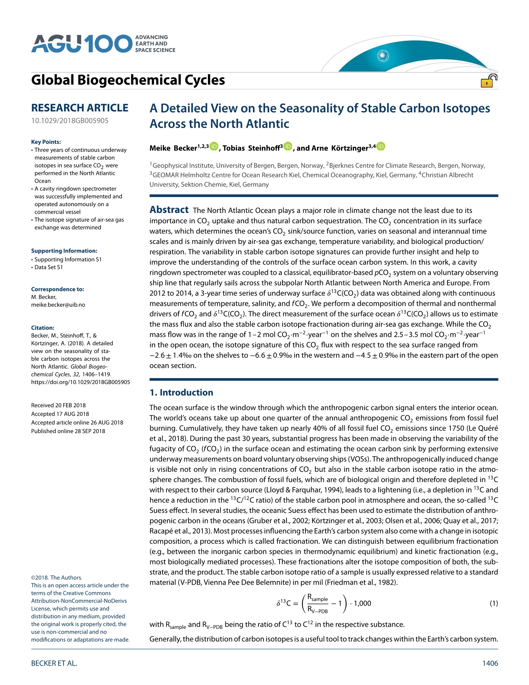
北大西洋在气候变化中发挥着重要作用,尤其是因为它对二氧化碳的吸收和自然碳的封存非常重要。其地表水中的二氧化碳浓度,随季节和年际时间尺度变化,主要受海气交换、温度变化和生物生产/呼吸的驱动,最终决定了海洋的二氧化碳汇/源功能。稳定碳同位素特征的变异性可以提供进一步的洞察,并有助于提高对表层海洋碳系统控制的理解。在这项工作中,一个光腔衰荡光谱仪(G2131-i)被耦合到一个经典的,基于平衡仪的pCO2系统上,这个系统安装在在北美和欧洲之间的亚极地北大西洋的一个定期航班上。2012年至2014年,在连续测量温度、盐度和fCO2的同时,获得了3年的航面δ13C(CO2)数据时间序列。我们对二氧化碳和 δ13C(CO2)进行热驱动和非热驱动分解。对表层海洋δ13C(CO2)的直接测量使我们能够估计质量流量,以及在海气交换过程中的稳定碳同位素分馏。当大陆架浅层上的二氧化碳质量流量在1–2 mol CO2⋅m−2⋅year−1和在开阔海域为2.5-3.5 mol CO2⋅m-2⋅year-1的范围内,CO2通量同位素特征为:海面的范围为-2.6±1.4‰,在西部为-6.6±0.9‰,在开阔海域东部为-4.5±0.9‰。
方案详情

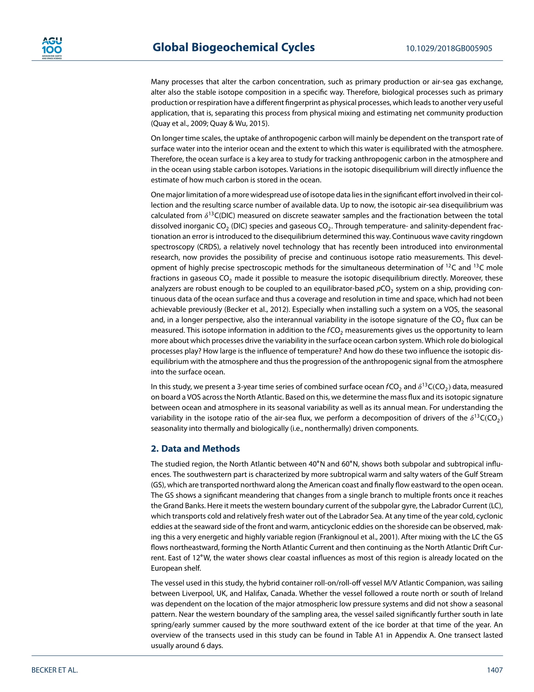
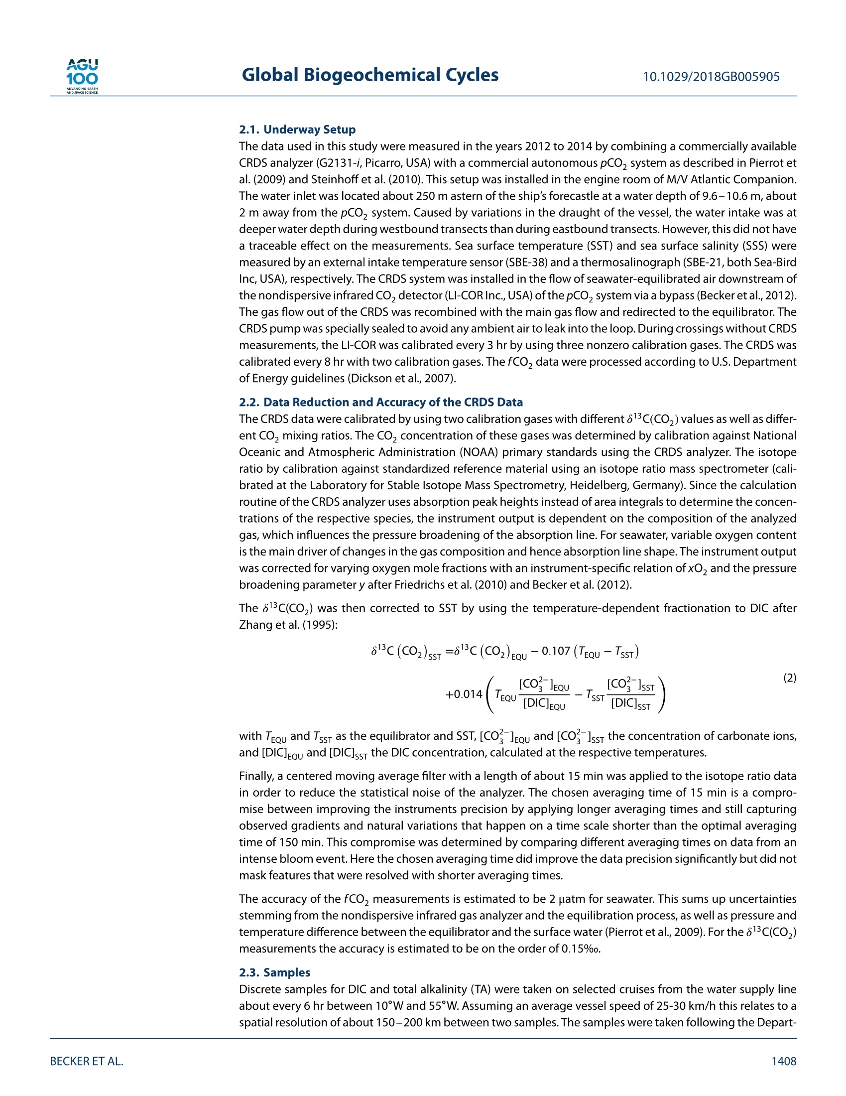
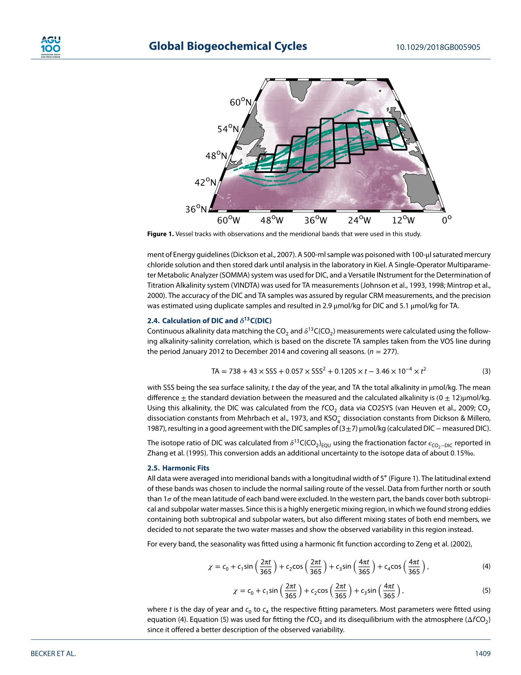
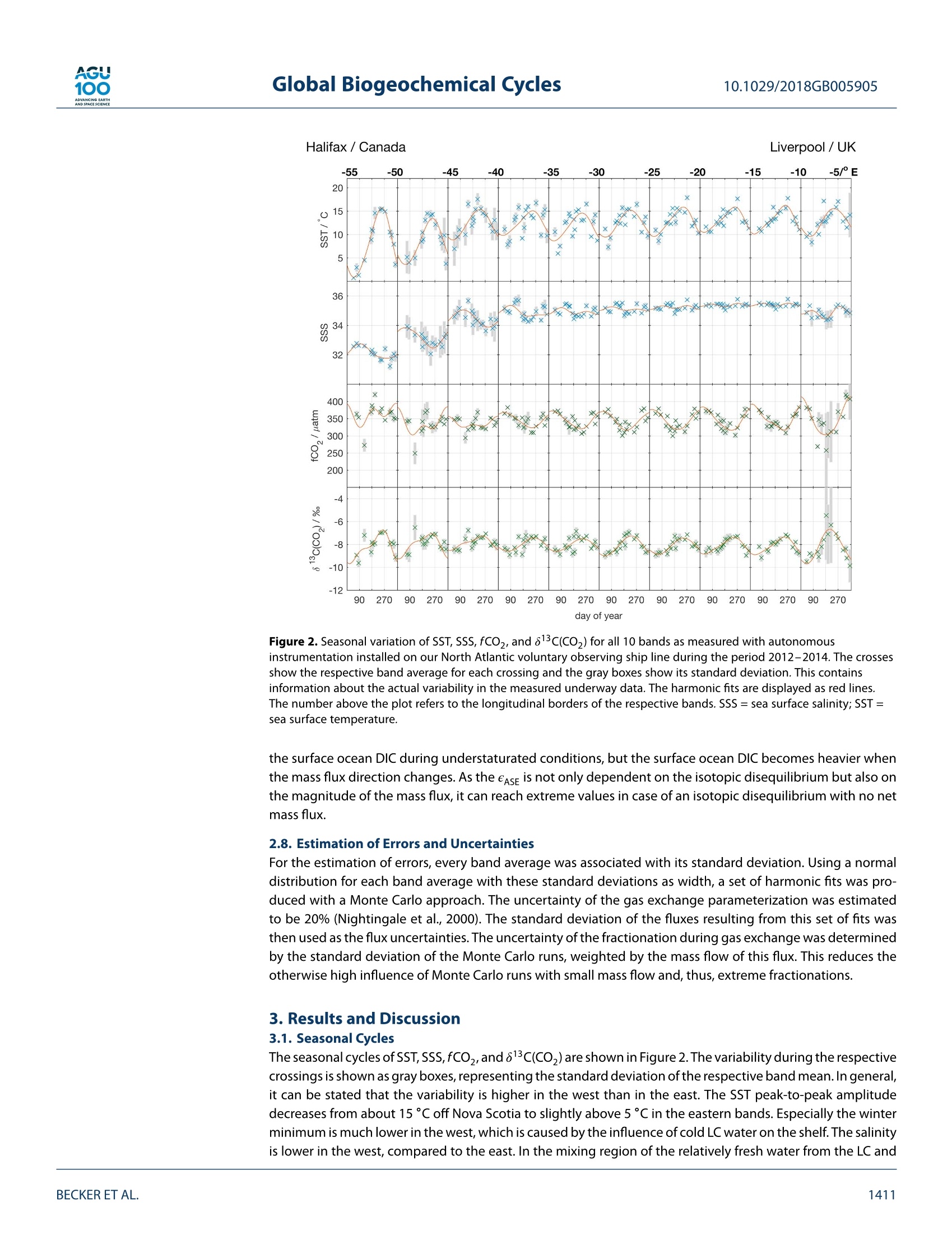
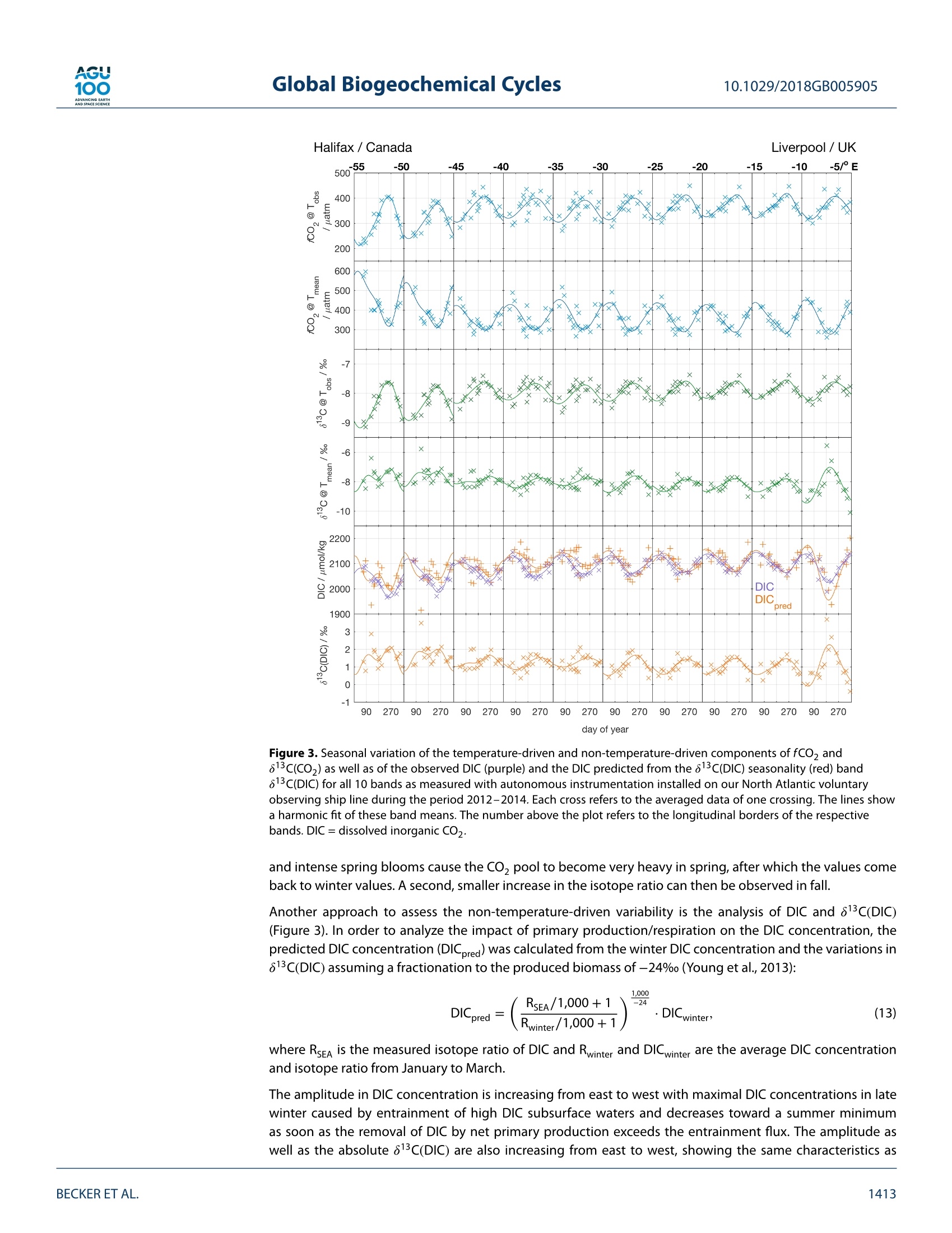
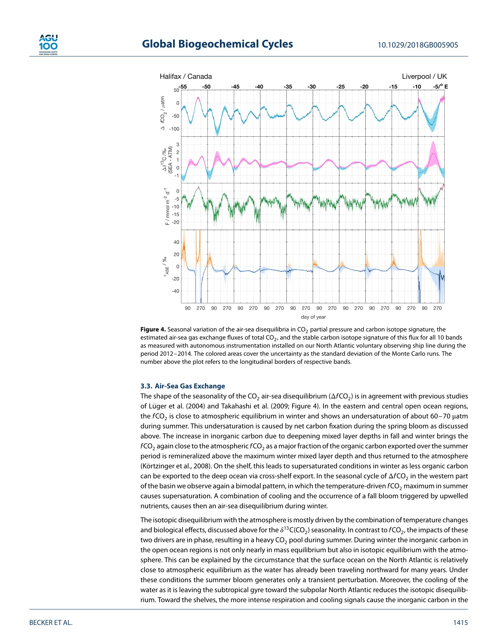
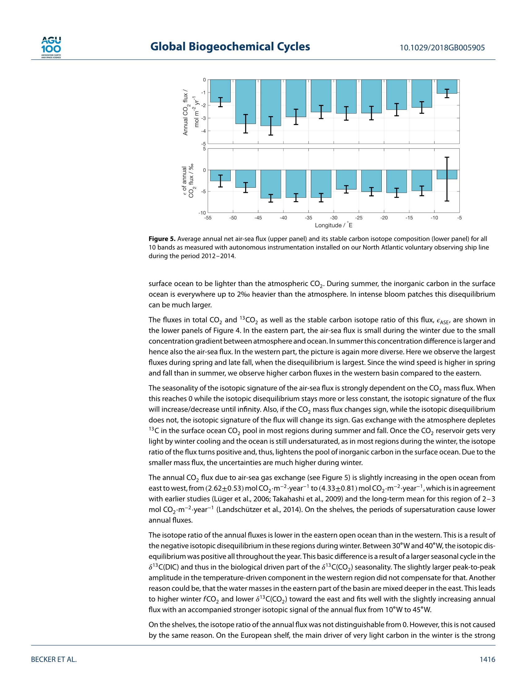
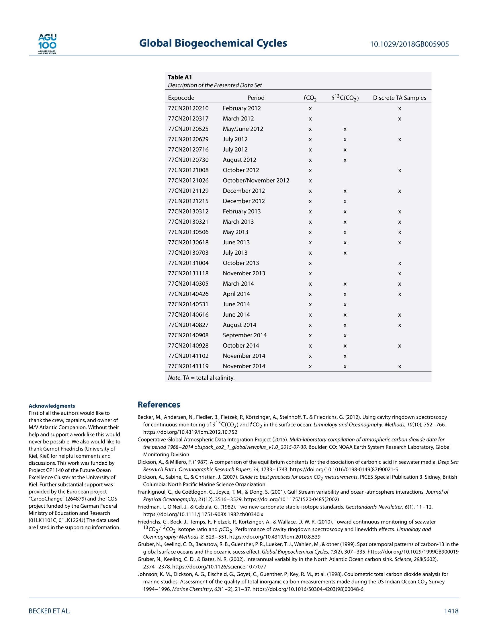
AGU100ADVANCINGEARTHANDSPACE SCIENCE Global Biogeochemical Cycles10.1029/2018GB005905 RESEARCH ARTICLE 10.1029/2018GB005905 Key Points: ·Three years of continuous underwaymeasurements of stable carbonisotopes in sea surface CO2 wereperformed in the North AtlanticOcean · A cavity ringdown spectrometerwas successfully implemented andoperated autonomously on acommercial vessel ·The isotope signature of air-sea gasexchange was determined Citation: https://doi.org/10.1029/2018GB005905 Received 20 FEB 2018 Accepted 17 AUG 2018 Accepted article online 26 AUG 2018 ◎2018. The Authors.This is an open access article under theterms of the Creative CommonsAttribution-NonCommercial-NoDerivsLicense, which permits use anddistribution in any medium, providedthe original work is properly cited, theuse is non-commercial and nomodifications or adaptations are made. A Detailed View on the Seasonality of Stable Carbon IsotopesAcross the North Atlantic Meike Becker1,2,3(3iD,Tobias SteinhoffiD, and Arne Kortzinger34 iD lGeophysical Institute, University of Bergen, Bergen, Norway,Bjerknes Centre for Climate Research, Bergen,Norway,3GEOMAR Helmholtz Centre for Ocean Research Kiel, Chemical Oceanography, Kiel, Germany, 4Christian AlbrechtUniversity, Sektion Chemie, Kiel,Germany Abstract The North Atlantic Ocean plays a major role in climate change not the least due to itsimportance in CO2 uptake and thus natural carbon sequestration. The CO2 concentration in its surfacewaters, which determines the ocean's CO, sink/source function, varies on seasonal and interannual timescales and is mainly driven by air-sea gas exchange, temperature variability, and biological production/respiration. The variability in stable carbon isotope signatures can provide further insight and help toimprove the understanding of the controls of the surface ocean carbon system. In this work, a cavityringdown spectrometer was coupled to a classical,equilibrator-based pCO, system on a voluntary observingship line that regularly sails across the subpolar North Atlantic between North America and Europe. From2012 to 2014, a 3-year time series of underway surface 813C(CO,) data was obtained along with continuousmeasurements of temperature, salinity,and fCO. We perform a decomposition of thermal and nonthermaldrivers of fCO, and 813C(CO,). The direct measurement of the surface ocean 813C(CO,) allows us to estimatethe mass flux and also the stable carbon isotope fractionation during air-sea gas exchange. While the CO,mass flow was in the range of 1-2 mol CO,·m-2.year- on the shelves and 2.5-3.5 mol CO,·m-2.year-1in the open ocean, the isotope signature of this CO, flux with respect to the sea surface ranged from-2.6±1.4%o on the shelves to -6.6±0.9%o in the western and -4.5±0.9%o in the eastern part of the openocean section. 1. Introduction The ocean surface is the window through which the anthropogenic carbon signal enters the interior ocean.The world's oceans take up about one quarter of the annual anthropogenic CO,emissions from fossil fuelburning. Cumulatively, they have taken up nearly 40% of all fossil fuel CO, emissions since 1750 (Le Quéréet al.,2018). During the past 30 years, substantial progress has been made in observing the variability of thefugacity of CO, (fCO,) in the surface ocean and estimating the ocean carbon sink by performing extensiveunderway measurements on board voluntary observing ships (VOSs). The anthropogenically induced changeis visible not only in rising concentrations of CO, but also in the stable carbon isotope ratio in the atmo-sphere changes. The combustion of fossil fuels, which are of biological origin and therefore depleted in 13Cwith respect to their carbon source (Lloyd & Farquhar, 1994), leads to a lightening (i.e., a depletion in 13C andhence a reduction in the 13C/12C ratio) of the stable carbon pool in atmosphere and ocean, the so-called 13cSuess effect. In several studies, the oceanic Suess effect has been used to estimate the distribution of anthro-pogenic carbon in the oceans (Gruber et al., 2002; Kortzinger et al., 2003; Olsen et al., 2006; Quay et al., 2017;Racapeet al., 2013). Most processes influencing the Earth's carbon system also come with a change in isotopiccomposition, a process which is called fractionation. We can distinguish between equilibrium fractionation(e.g., between the inorganic carbon species in thermodynamic equilibrium) and kinetic fractionation (e.g.,most biologically mediated processes). These fractionations alter the isotope composition of both, the sub-strate, and the product. The stable carbon isotope ratio of a sample is usually expressed relative to a standardmaterial (V-PDB, Vienna Pee Dee Belemnite) in per mil (Friedman et al.,1982). with Rsample and Ry-PDB being the ratio of C13 to C12 in the respective substance. Many processes that alter the carbon concentration, such as primary production or air-sea gas exchange,alter also the stable isotope composition in a specific way. Therefore, biological processes such as primaryproduction or respiration have a different fingerprint as physical processes, which leads to another very usefulapplication, that is, separating this process from physical mixing and estimating net community production(Quay et al., 2009; Quay &Wu, 2015). On longer time scales, the uptake of anthropogenic carbon will mainly be dependent on the transport rate ofsurface water into the interior ocean and the extent to which this water is equilibrated with the atmosphere.Therefore, the ocean surface is a key area to study for tracking anthropogenic carbon in the atmosphere andin the ocean using stable carbon isotopes. Variations in the isotopic disequilibrium will directly influence theestimate of how much carbon is stored in the ocean. Onemajor limitation of a more widespread use of isotope data lies in the significant effort involved in their col-lection and the resulting scarce number of available data. Up to now, the isotopic air-sea disequilibrium wascalculated from 813C(DIC) measured on discrete seawater samples and the fractionation between the totaldissolved inorganic COz(DIC) species and gaseous CO,. Through temperature-and salinity-dependent frac-tionation an error is introduced to the disequilibrium determined this way. Continuous wave cavity ringdownspectroscopy (CRDS), a relatively novel technology that has recently been introduced into environmentalresearch, now provides the possibility of precise and continuous isotope ratio measurements. This devel-opment of highly precise spectroscopic methods for the simultaneous determination of 12C and 13C molefractions in gaseous CO, made it possible to measure the isotopic disequilibrium directly. Moreover, theseanalyzers are robust enough to be coupled to an equilibrator-based pCO, system on a ship, providing con-tinuous data of the ocean surface and thus a coverage and resolution in time and space, which had not beenachievable previously (Becker et al., 2012). Especially when installing such a system on a VOS, the seasonaland, in a longer perspective, also the interannual variability in the isotope signature of the CO, flux can bemeasured. This isotope information in addition to the fCO, measurements gives us the opportunity to learnmore about which processes drive the variability in the surface ocean carbon system. Which role do biologicalprocesses play? How large is the influence of temperature? And how do these two influence the isotopic dis-equilibrium with the atmosphere and thus the progression of the anthropogenic signal from the atmosphereinto the surface ocean. In this study, we present a 3-year time series of combined surface ocean fCO, and 813C(CO,) data, measuredon board a VOS across the North Atlantic. Based on this, we determine the mass flux and its isotopic signaturebetween ocean and atmosphere in its seasonal variability as well as its annual mean. For understanding thevariability in the isotope ratio of the air-sea flux, we perform a decomposition of drivers of the 813C(CO))seasonality into thermally and biologically (i.e., nonthermally) driven components. 2. Data and Methods The studied region, the North Atlantic between 40°N and 60°N, shows both subpolar and subtropical influ-ences. The southwestern part is characterized by more subtropical warm and salty waters of the Gulf Stream(GS), which are transported northward along the American coast and finally flow eastward to the open ocean.The GS shows a significant meandering that changes from a single branch to multiple fronts once it reachesthe Grand Banks. Here it meets the western boundary current ofthe subpolar gyre, the Labrador Current (LC),which transports cold and relatively fresh water out of the Labrador Sea. At any time of the year cold, cycloniceddies at the seaward side of the front and warm, anticyclonic eddies on the shoreside can be observed, mak-ing this a very energetic and highly variable region (Frankignoul et al., 2001). After mixing with the LC the GSflows northeastward, forming the North Atlantic Current and then continuing as the North Atlantic Drift Cur-rent. East of 12°W, the water shows clear coastal influences as most of this region is already located on theEuropean shelf. The vessel used in this study, the hybrid container roll-on/roll-off vessel M/V Atlantic Companion, was sailingbetween Liverpool, UK, and Halifax, Canada. Whether the vessel followed a route north or south of Irelandwas dependent on the location of the major atmospheric low pressure systems and did not show a seasonalpattern. Near the western boundary of the sampling area, the vessel sailed significantly further south in latespring/early summer caused by the more southward extent of the ice border at that time of the year. Anoverview of the transects used in this study can be found in Table A1 in Appendix A. One transect lastedusually around 6 days. 2.1. Underway Setup The data used in this study were measured in the years 2012 to 2014 by combining a commercially availableCRDS analyzer (G2131-i, Picarro, USA) with a commercial autonomous pCO, system as described in Pierrot etal. (2009) and Steinhoff et al. (2010). This setup was installed in the engine room of M/V Atlantic Companion.The water inlet was located about 250 m astern of the ship's forecastle at a water depth of 9.6-10.6 m, about2 m away from the pCo, system. Caused by variations in the draught of the vessel, the water intake was atdeeper water depth during westbound transects than during eastbound transects. However, this did not havea traceable effect on the measurements. Sea surface temperature (SST) and sea surface salinity (SSS) weremeasured by an external intake temperature sensor (SBE-38) and a thermosalinograph (SBE-21, both Sea-BirdInc, USA), respectively. The CRDS system was installed in the flow of seawater-equilibrated air downstream ofthe nondispersive infrared CO, detector (LI-CORInc.,USA) of thepCO, system via a bypass (Beckeret al.,2012).The gas flow out of the CRDS was recombined with the main gas flow and redirected to the equilibrator. TheCRDS pump was specially sealed to avoid any ambient air to leak into the loop. During crossings without CRDSmeasurements, the LI-COR was calibrated every 3 hr by using three nonzero calibration gases. The CRDS wascalibrated every 8 hr with two calibration gases. The fCO, data were processed according to U.S. Departmentof Energy guidelines (Dickson et al., 2007). 2.2. Data Reduction and Accuracy of the CRDS Data The CRDS data were calibrated by using two calibration gases with different 813c(CO,) values as well as differ-ent CO, mixing ratios. The CO,concentration of these gases was determined by calibration against NationalOceanic and Atmospheric Administration (NOAA) primary standards using the CRDS analyzer. The isotoperatio by calibration against standardized reference material using an isotope ratio mass spectrometer (cali-brated at the Laboratory for Stable Isotope Mass Spectrometry, Heidelberg, Germany). Since the calculationroutine of the CRDS analyzer uses absorption peak heights instead of area integrals to determine the concen-trations of the respective species, the instrument output is dependent on the composition of the analyzedgas, which influences the pressure broadening of the absorption line. For seawater, variable oxygen contentis the main driver of changes in the gas composition and hence absorption line shape. The instrument outputwas corrected for varying oxygen mole fractions with an instrument-specific relation ofx0, and the pressurebroadening parameter y after Friedrichs et al. (2010) and Becker et al. (2012). The 813C(CO)) was then corrected to SST by using the temperature-dependent fractionation to DIC afterZhang et al.(1995): with TeQu and Tssr as the equilibrator and SST, [CO,]equ and [CO,lssr the concentration of carbonate ions,and [DIC]EQu and [DIC]ssr the DIC concentration, calculated at the respective temperatures. Finally, a centered moving average filter with a length of about 15 min was applied to the isotope ratio datain order to reduce the statistical noise of the analyzer. The chosen averaging time of 15 min is a compro-mise between improving the instruments precision by applying longer averaging times and still capturingobserved gradients and natural variations that happen on a time scale shorter than the optimal averagingtime of 150 min. This compromise was determined by comparing different averaging times on data from anintense bloom event. Here the chosen averaging time did improve the data precision significantly but did notmask features that were resolved with shorter averaging times. The accuracy of the fCO, measurements is estimated to be 2 uatm for seawater. This sums up uncertaintiesstemming from the nondispersive infrared gas analyzer and the equilibration process, as well as pressure andtemperature difference between the equilibrator and the surface water (Pierrot et al., 2009). For the813C(CO,)measurements the accuracy is estimated to be on the order of 0.15%o. Discrete samples for DIC and total alkalinity (TA) were taken on selected cruises from the water supply lineabout every 6 hr between 10°W and 55°W. Assuming an average vessel speed of 25-30 km/h this relates to aspatial resolution of about 150-200 km betweentwo samples. The samples were taken following the Depart- 0° Figure 1. Vessel tracks with observations and the meridional bands that were used in this study. ment of Energy guidelines (Dickson et al.,2007). A500-ml samplewas poisoned with 100-pl saturated mercurychloride solution and then stored dark until analysis in the laboratory in Kiel. A Single-Operator Multiparame-ter Metabolic Analyzer (SOMMA) system was used for DIC, and a Versatile INstrument for the Determination ofTitration Alkalinity system (VINDTA) was used for TA measurements (Johnson et al., 1993,1998; Mintrop et al.,2000). The accuracy of the DIC and TA samples was assured by regular CRM measurements, and the precisionwas estimated using duplicate samples and resulted in 2.9 umol/kg for DIC and 5.1 umol/kg for TA. 2.4. Calculation of DIC and 813C(DIC) Continuous alkalinity data matching the CO, and 813c(CO,) measurements were calculated using the follow-ing alkalinity-salinity correlation,which is based on the discrete TA samples taken from the VOS line duringthe period January 2012 to December 2014 and covering all seasons. (n=277). with SSS being the sea surface salinity, t the day of the year, and TA the total alkalinity in umol/kg. The meandifference ± the standard deviation between the measured and the calculated alkalinity is (0±12)umol/kg.Using this alkalinity, the DIC was calculated from the fCO, data via CO2SYS (van Heuven et al., 2009; CO,dissociation constants from Mehrbach et al., 1973, and KSO-dissociation constants from Dickson & Millero,1987), resulting in a good agreement with the DIC samples of (3±7) umol/kg (calculated DIC- measured DIC). The isotope ratio of DIC was calculated from 813C(CO2)Eou using the fractionation factor eco,-Dic reported inZhang et al. (1995). This conversion adds an additional uncertainty to the isotope data of about 0.15%o. 2.5. Harmonic Fits All data were averaged into meridional bands with a longitudinal width of 5° (Figure 1). The latitudinal extendof these bands was chosen to include the normal sailing route of the vessel. Data from further north or souththan 1o of the mean latitude of each band were excluded. In the western part, the bands cover both subtropi-cal and subpolar water masses. Since this is a highly energetic mixing region, in which we found strong eddiescontaining both subtropical and subpolar waters, but also different mixing states of both end members, wedecided to not separate the two water masses and show the observed variability in this region instead. For every band, the seasonality was fitted using a harmonic fit function according to Zeng et al. (2002), where t is the day of year and co to ca the respective fitting parameters. Most parameters were fitted usingequation (4). Equation (5) was used for fitting the fCO, and its disequilibrium with the atmosphere (AfCO,)since it offered a better description of the observed variability. 2.6. Decomposition of Driving Factors The temperature-driven and the non-temperature-driven components of the fCo, (fCOz@Tobs andfCO,@Tmean) were calculated after Takahashi et al.,1993 (1993; equations (6) and (7)). Since the stable carbonisotope ratio of DIC as a conservative property is constant with temperature,the decomposition of 813C(CO,)can be based on the temperature-dependent fractionation between DIC and CO,(equations (8) and (9)). 813c(Coz)@Tobs=813c(C02)mean -0.107 (Tmean-Tobs) (8) 813c (Coz)@Tmean =83c(C02)obs-0.107 (Tobs-Tmean) The subscript obs refers to the observed values, while the subscript mean refers to the respective annual mean. 2.7. Air-Sea Gas Exchange The atmospheric fCo, (fCO2.ATM) and 813C(CO2)ATM were calculated for each meridional band based ontime series measurements from atmosphere monitoring stations at Mace Head, Ireland (53.33°N,-9.90°E);Bermuda, UK (32.26°N, -64.88°E); Vestmannaeyjar, Iceland (63.40°N, 20.29°E); and the Azores, Portugal(38.75°N,-27.08°E) between January 2012 and December 2014 (Cooperative Global Atmospheric Data Inte-gration Project, 2015; White et al.,2015). Since the atmospheric CO, content shows a strong latitudinaldependence, this dependence was used to calculate the atmosphericxCO, and 813C(CO,)ATM over the oceanas a function of latitude and date. All grid points within the respective latitude were averaged to one meanseasonal cycle per band. The fCo y was calculated from the xCOATy using the harmonic fits of SST, SSS,and air pressure. Wind speed data were taken from the Modern Era Retrospective-analysis for Research and Applications, ver-sion 2, which uses the Goddard Earth Observing System Data Assimilation System, version 5. The barometricpressure as obtained from this reanalysis was in good agreement with our measurements on board. The gastransfer velocity k6oo was calculated according to Nightingale et al. (2000) for the entire wind field. The gastransfer velocity was then averaged into a daily mean per band, and a 6-day moving average was applied.The actual k at the respective temperatures was calculated using the Schmidt number dependence after.Wanninkhof (1992) and the solubility coefficient K, according to Weiss (1974). The sea-to-air flux of total CO (F) and 13Co (F13) was calculated using equations (10) to (12) where K is the solubility of CO, in seawater, k the gas transfer velocity, a the fractionation during gasexchange, and Rse and RATy the respective stable carbon isotope ratios of CO, in seawater and the atmo-sphere (calculated after equation (1)). Please note that eAse describes the isotopic composition of the flux between atmosphere and ocean relativeto the isotopic composition of the surface ocean. A negative eAse means that the gas exchange is lightening Halifax / Canada Liverpool/UK Figure 2. Seasonal variation of SST, SSS, fCO,and 813c(CO)) for all 10 bands as measured with autonomousinstrumentation installed on our North Atlantic voluntary observing ship line during the period 2012-2014. The crossesshow the respective band average for each crossing and the gray boxes show its standard deviation. This containsinformation about the actual variability in the measured underway data. The harmonic fits are displayed as red lines.The number above the plot refers to the longitudinal borders of the respective bands. SSS = sea surface salinity; SST =sea surface temperature. the surface ocean DIC during understaturated conditions, but the surface ocean DIC becomes heavier whenthe mass flux direction changes. As the ease is not only dependent on the isotopic disequilibrium but also onthe magnitude of the mass flux, it can reach extreme values in case of an isotopic disequilibrium with no netmass flux. 2.8. Estimation of Errors and Uncertainties For the estimation of errors,every band average was associated with its standard deviation. Using a normaldistribution for each band average with these standard deviations as width,a set of harmonic fits was pro-duced with a Monte Carlo approach. The uncertainty of the gas exchange parameterization was estimatedto be 20% (Nightingale et al., 2000). The standard deviation of the fluxes resulting from this set of fits wasthen used as the flux uncertainties. The uncertainty of the fractionation during gas exchange was determinedby the standard deviation of the Monte Carlo runs, weighted by the mass flow of this flux. This reduces theotherwise high influence of Monte Carlo runs with small mass flow and, thus, extreme fractionations. 3. Results and Discussion 3.1. Seasonal Cycles The seasonal cycles of SST,SSS,fCO,,and813C(CO,)are shown in Figure 2. The variability during the respectivecrossings is shown as gray boxes, representing the standard deviation of the respective band mean. In general,it can be stated that the variability is higher in the west than in the east. The SST peak-to-peak amplitudedecreases from about 15 °C off Nova Scotia to slightly above 5C in the eastern bands. Especially the winterminimum is much lower in the west, which is caused by the influence of cold LC water on the shelf. The salinityis lower in the west, compared to the east. In the mixing region of the relatively fresh water from the LC and the saline GS water between 35°W and 50°W, high variability was found. In the salinity data, we can observea small seasonal cycle with higher salinities in late winter and a minimum in fall. The observed patterns in fCO, seasonality across the North Atlantic are well described in the literature(Lugeret al., 2004;Takahashi et al.,2009). The region east of 40°W shows a seasonality that is more typical for subpolarregions. A distinct decrease toward a summer minimum due to primary production is followed by an increasecaused by convective mixing in fall and winter. The amplitude is increasing toward the east from about 50 to80 uatm. The easternmost region, between 5°W and 10°W, is located on the shelf, showing high spatial vari-ability during summer, which can be seen in the high standard deviation of the band averages. Very intenseblooms in spring were followed by also intense respiration signals ventilated through the deepening mixedlayer depth in the end of summer. In contrast, the western part shows a bimodal pattern that points towardsubtropical influences. The data show an early minimum in spring caused by carbon fixation, during whichthe fCO, can easily be reduced to less than 250 patm, followed by a temperature-driven maximum during thesummer months, which decreases again toward fall. These waters at the front of LC and GS and at the shelfedge of the Grand Banks can be very patchy. The further west,the more pronounced is the subtropical pattern.While there is still a maximum in winter around 45°W,the summer maximum dominates west of 50°W. The seasonality of 813c(CO,) also shows basic differences between east and west. In the eastern half of theNorth Atlantic, the seasonal cycle of 813C(CO,) is anticorrelated to fCO. The carbon pool becomes heavier aslight carbon is preferably taken up by phytoplankton during spring bloom, while upward mixing of respiratorycarbon depletes in 13c in the inorganic carbon pool again in fall. In the western part, the anticorrelation is lesspronounced and the 813C(CO,) seasonality has two maxima, one during spring bloom and one in late summer.At the frontal region of LC and GS, this enrichment in 13C can lead to 813C(CO,) values higher than -4%o thatare usually not observed in the open ocean, correlated to the extraordinarily low fCO,observed in that area. 3.2. Decomposition of Temperature and Nontemperature Effects Since fCO, has a strong temperature dependence, it is often decomposed into a temperature-dependent andnon-temperature-dependent component (Takahashi et al., 1993). Note that this decomposition assumes noair-sea exchange of CO,. This assumption is not strictly valid but generally justified as the CO, equilibrationtime scale of the surface ocean (1 year) is long to the time scales of the seasonal cyles of temperature andnet community production. For the data set presented here, this analysis is shown in the upper two panels ofFigure 3. The temperature-driven part, fCO,@ Tos, shows a minimum in winter and a maximum in summer,with an amplitude decreasing from west to east. This effect is caused by the temperature-dependent solu-bility of CO,. The non-temperature-driven part of the fCO, seasonality, fCO,@ Tmean, has an opposite shape.This part contains biological effects: convection and advection. In the temperate North Atlantic, the balanceof primary production and respiration is a major driver of fCO,. The onset of primary production in springdraws down the fCo,@ Tmean, while the upward mixing of carbon-rich water during fall leads to increasingfCO, @ Tmean· The amplitude of fCO, @ Tmean is slightly higher on the shelves, especially in the west, wheremore intense primary production takes place but does not show a clear longitudinal trend. As a result of this,both components, fCO,@ Tmean and fCO@ Tobs, are of similar magnitude in the western bands, while thenon-temperature-driven part is dominating in the east, manifesting the eastward transition from subtropicalto more subpolar character of the surface ocean dynamics. When looking at the decomposition of the seasonality of stable carbon isotope ratios, the main difference tothat ofthe fCO, seasonality is that both forcings have the same direction in their effect on 813C(CO,).813C(CO2)@ Tobs shows a summer maximum and winter minimum with an amplitude of 1.5%o in the west, decreasingto about 1% in the eastern part. This variability results from the temperature-dependent equilibrium frac-tionation within the inorganic carbon system. At higher temperatures the fractionation between CO, and theDIC pool is reduced, leading to higher isotope ratios in the measured CO, (about 2%o per 10C [Zhang et al.,1995]). The non-temperature-driven part of the 813c(CO,) seasonality (813C(CO,) @ Tmean) shows more vari-ability. Generally, during carbon fixation by phytoplankton the lighter isotopomer is preferred due to kineticfractionation. This results in an enrichment of the heavier isotopomer in the remaining carbon pool in thesurface ocean. During respiration, most of the light biomass is remineralized completely, so that the isotoperatio of inorganic carbon decreases again when remineralized carbon and nutrients are mixed to the surfaceduring convective mixing. East of 35°W the 813C(CO)@ Tmean seasonality shows an amplitude of about 1%oin the open ocean and a larger amplitude in the shelf. West of 35°W, bimodal patterns are observed. The early Halifax/Canada Figure 3. Seasonal variation of the temperature-driven and non-temperature-driven components of fCO2 and 813C(CO,) as well as of the observed DIC (purple) and the DIC predicted from the 813C(DIC) seasonality (red) band813C(DIC) for all 10 bands as measured with autonomous instrumentation installed on our North Atlantic voluntaryobserving ship line during the period 2012-2014. Each cross refers to the averaged data of one crossing. The lines showa harmonic fit of these band means. The number above the plot refers to the longitudinal borders of the respectivebands. DIC= dissolved inorganic CO,. and intense spring blooms cause the CO, pool to become very heavy in spring, after which the values comeback to winter values. A second, smaller increase in the isotope ratio can then be observed in fall. Another approach to assess the non-temperature-driven variability is the analysis of DIC and 813C(DIC)(Figure 3). In order to analyze the impact of primary production/respiration on the DIC concentration, thepredicted DIC concentration (DICpred) was calculated from the winter DIC concentration and the variations in813C(DIC) assuming a fractionation to the produced biomass of -24% (Young et al., 2013): where RsEA is the measured isotope ratio of DIC and Rwinter and DICwinter are the average DIC concentrationand isotope ratio from January to March. The amplitude in DIC concentration is increasing from east to west with maximal DIC concentrations in latewinter caused by entrainment of high DIC subsurface waters and decreases toward a summer minimumas soon as the removal of DIC by net primary production exceeds the entrainment flux. The amplitude aswell as the absolute 813C(DIC) are also increasing from east to west, showing the same characteristics as the non-temperature-driven component of the 813C(CO)). In the eastern open ocean bands (10-30°W), it isclearly anticorrelated to the changes in DIC concentration. The amplitude in DIC concentration is about 80umol/kg, while that in 813C(DIC) shows about 1%o. The predicted DIC concentration based on the assumption that only primary production and respiration drivethe seasonal DIC variability shows a very similar amplitude and timing as the actually measured DIC concen-tration. So both the DIC and 813C(DIC) changes are almost completely biologically driven. This fits well withother studies in the subpolar North Atlantic (Gruber et al., 1999;Racape et al.,2014). The easternmost band,which is located around the coast of Ireland,shows a larger but still anticorrelated amplitude in both DIC con-centration and its stable isotope composition (120 umol/kg,2%). The predicted DIC variations based on the813C(DIC) seasonality show a larger amplitude than the actually measured DIC concentration. This leads to theconclusion that there must be a different source of DIC, for example, fluxes from land or the seafloor, whichmost likely also carry an isotope composition different to that of surface ocean DIC or phytoplankton biomass. The picture in the western bands is more complicated, however. The decrease in DIC starts earlier and issteeper in the western part of the basin, while the net entrainment flux starts later in the season as in theeastern open ocean regions. The minimal DIC concentration is reached in August. In these bands the har-monic fit performs not very well in capturing the first steep decline in DIC concentration/increase in 813C(DIC),but when looking at the measured values themselves, it becomes visible that the first decrease in DIC inspring bloom of about 80 umol/kg happens within only 50 days in March/April, associated with an increase in813C(DIC) of 2%0. This region is known to show a nitrate-depleted conditions from June to August (Steinhoff et al.,2010). The813C(DIC) shows a bimodal structure with one maximum at the time of the first steep DIC drawdown undernitrate-repleted conditions in spring and a second maximum coinciding with the DIC minimum in late sum-mer. This behavior can be explained by two different processes. This region is characterized by oligotrophicconditions and very shallow mixed layer depths during summer. In spring, the available nutrients are usedup during a short but intense bloom phase, leading to the first maximum in 813C(DIC). The lower 813C afterthe end of spring bloom could be caused by the ingassing of lighter atmospheric carbon, which can havea large influence on surface layer 813C(DIC) during shallow mixed layer conditions. A different process thatcould introduce light carbon into the surface ocean is remineralization. Especially, if this remineralization isnot occurring quantitatively in the surface layer, light carbon would be released in the surface layer due to thispartial remineralization, while the remaining, relatively heavy particles would sink out of the mixed layer.Khimet al.(2018) found heavier sinking particles during the highly productive seasons. Usually, this is connectedto changes in the 813C of dissolved CO, but in a region with a high rate of remineralized production and ashallow mixed layer as the western part of the area studied here is during summer, a partial remineralizationas source of light carbon needs to be considered. The further DIC decrease toward the overall minimum coin-cides with a decrease in salinity at the same time of the year and the onset of mixed layer deepening in fall. Thisdecrease is coming with an increase in 813C(DIC), showing a biological signature (about 0.5%o per 40 umol/kgdecrease in DIC). As the decrease in DIC is associated with a lower salinity, this signature must be caused bymixing with lower salinity water, which comes with a different isotopic signature and which has experienceda DIC decrease caused by a phytoplankton bloom. The decrease in salinity is a seasonal signature that occurssimultaneously with the onset of convective mixing. Since the MLD in this region is very shallow during sum-mer, evaporation could increase the salinity in the surface layer, so that mixed layer deepening can cause adecrease in salinity.Additionally, increased precipitation during fall would lead to a decrease in salinity. Afterthe cessation of the spring bloom there can be a significant amount of primary production occurring under-neath the very shallow mixed layer where the nutrient concentration is not yet fully depleted and light levelstill permit net primary production. Mixing with this shallow subsurface water mass that is not influenced byair sea gas exchange could provide persistent primary production signal in the 813C(DIC). Subsurface bloomsin midsummer with a deep chlorophyll maximum are reported for subtropical regions and consume nutri-ents near the nutricline below the shallow summer mixed layer. This scenario is consistent with the delay ofa net entrainment flux of nutrients relative to the onset of deepening of the mixed layer and can explain theobserved pattern. Another process that could possibly cause such a signature would be a fall bloom that pro-duces the biological isotope signature and coincides with lateral mixing of lower salinity waters that wereinfluenced by ice melting in summer. Halifax / Canada Liverpool/UK Figure 4. Seasonal variation of the air-sea disequilibria in CO2 partial pressure and carbon isotope signature,theestimated air-sea gas exchange fluxes of total CO2, and the stable carbon isotope signature of this flux for all 10 bandsas measured with autonomous instrumentation installed on our North Atlantic voluntary observing ship line during theperiod 2012-2014. The colored areas cover the uncertainty as the standard deviation of the Monte Carlo runs. Thenumber above the plot refers to the longitudinal borders of respective bands. 3.3. Air-Sea Gas Exchange The shape of the seasonality of the CO, air-sea disequilibrium (AfCO,) is in agreement with previous studiesof Luger et al. (2004) and Takahashi et al. (2009; Figure 4). In the eastern and central open ocean regions,the fCO, is close to atmospheric equilibrium in winter and shows an undersaturation of about 60-70 uatmduring summer. This undersaturation is caused by net carbon fixation during the spring bloom as discussedabove. The increase in inorganic carbon due to deepening mixed layer depths in fall and winter brings thefCO, again close to the atmospheric fCO, as a major fraction of the organic carbon exported over the summerperiod is remineralized above the maximum winter mixed layer depth and thus returned to the atmosphere(Kortzinger et al., 2008). On the shelf, this leads to supersaturated conditions in winter as less organic carboncan be exported to the deep ocean via cross-shelf export. In the seasonal cycle of AfCO, in the western partof the basin we observe again a bimodal pattern, in which the temperature-driven fCO, maximum in summercauses supersaturation. A combination of cooling and the occurrence of a fall bloom triggered by upwellednutrients, causes then an air-sea disequilibrium during winter. The isotopic disequilibrium with the atmosphere is mostly driven by the combination of temperature changesand biological effects, discussed above for the 813c(CO,) seasonality. In contrast to fCo, the impacts of thesetwo drivers are in phase, resulting in a heavy CO, pool during summer. During winter the inorganic carbon inthe open ocean regions is not only nearly in mass equilibrium but also in isotopic equilibrium with the atmo-sphere. This can be explained by the circumstance that the surface ocean on the North Atlantic is relativelyclose to atmospheric equilibrium as the water has already been traveling northward for many years.Underthese conditions the summer bloom generates only a transient perturbation. Moreover, the cooling of thewater as it is leaving the subtropical gyre toward the subpolar North Atlantic reduces the isotopic disequilib-rium. Toward the shelves, the more intense respiration and cooling signals cause the inorganic carbon in the Figure 5. Average annual net air-sea flux (upper panel) and its stable carbon isotope composition (lower panel) for all10 bands as measured with autonomous instrumentation installed on our North Atlantic voluntary observing ship lineduring the period 2012-2014. surface ocean to be lighter than the atmospheric CO,.During summer, the inorganic carbon in the surfaceocean is everywhere up to 2% heavier than the atmosphere. In intense bloom patches this disequilibriumcan be much larger. The fluxes in total Co, and 13co, as well as the stable carbon isotope ratio of this flux, eAse, are shown inthe lower panels of Figure 4. In the eastern part, the air-sea flux is small during the winter due to the smallconcentration gradient between atmosphere and ocean.In summerthis concentration difference is larger andhence also the air-sea flux. In the western part, the picture is again more diverse. Here we observe the largestfluxes during spring and late fall, when the disequilibrium is largest. Since the wind speed is higher in springand fall than in summer, we observe higher carbon fluxes in the western basin compared to the eastern. The seasonality of the isotopic signature of the air-sea flux is strongly dependent on the CO, mass flux. Whenthis reaches 0 while the isotopic disequilibrium stays more or less constant, the isotopic signature of the fluxwill increase/decrease until infinity. Also, if the CO, mass flux changes sign, while the isotopic disequilibriumdoes not, the isotopic signature of the flux will change its sign. Gas exchange with the atmosphere depletes13C in the surface ocean CO, pool in most regions during summer and fall. Once the CO, reservoir gets verylight by winter cooling and the ocean is still undersaturated, as in most regions during the winter, the isotoperatio of the flux turns positive and,thus, lightens the pool of inorganic carbon in the surface ocean. Due to thesmaller mass flux, the uncertainties are much higher during winter. The annual CO, flux due to air-sea gas exchange (see Figure 5) is slightly increasing in the open ocean fromeast to west, from (2.62±0.53)molCO·m-2.year-to(4.33±0.81)molCO,·m-2.year-,which is in agreementwith earlier studies (Luger et al., 2006; Takahashi et al., 2009) and the long-term mean for this region of 2-3mol CO,·m-2.year-1 (Landschutzer et al.,2014). On the shelves, the periods of supersaturation cause lowerannual fluxes. The isotope ratio of the annual fluxes is lower in the eastern open ocean than in the western. This is a result ofthe negative isotopic disequilibrium in these regions during winter. Between 30°W and 40°W, the isotopic dis-equilibrium was positive all throughout the year. This basic difference is a result of a larger seasonal cycle in the813C(DIC) and thus in the biological driven part of the 813c(CO,) seasonality. The slightly larger peak-to-peakamplitude in the temperature-driven component in the western region did not compensate for that. Anotherreason could be, that the water masses in the eastern part of the basin are mixed deeper in the east. This leadsto higher winter fCo, and lower 813C(CO,) toward the east and fits well with the slightly increasing annualflux with an accompanied stronger isotopic signal of the annual flux from 10°W to 45°W. On the shelves, the isotope ratio of the annual flux was not distinguishable from 0. However, this is not causedby the same reason. On the European shelf, the main driver of very light carbon in the winter is the strong biological cycle (see Figure 3). In contrast to that, temperature variations play the major role in the Great Bankregion. The strong winter cooling reduces the 813C(CO) in the surface ocean under that of the overlayingatmosphere. 4. Conclusion We successfully added a CRDS system to an existing autonomous underway fCO, system on a voluntaryobserving ship and can present now a unique 3-year time series of surface water fCO, and 813c(CO). Whilethe use of VOS is established for fCO, measurements on different routes in this region, this implementationis new for 813C(CO,). The now available resolution in time and space gives us the possibility to close the datagap in winter and study regional differences in the seasonality of 813C of gaseous CO, in seawater as wellas, calculated from this, the 813C(DIC). The direct comparison to the existing 813C(DIC) data sets is limited bythe calculation of the fraction factor between DIC and gaseous CO. As this kind of instruments will mostlikely be more widely used in the future, we strongly want to encourage to conduct a new estimation of thetemperature, salinity, and pH sensitivity of this fractionation factor. We used this time series to perform a decomposition of the 813c(CO,) seasonality with respect to the driv-ing factors temperature and biology. This decomposition revealed a dominantly biological-driven cycle inthe east, while temperature becomes more dominant toward the west. This shift was much clearer in the813c(CO,) seasonality than in that of fCO. Another interesting pattern that could be observed in the west-ern, subtropical part of the basin was the bimodal pattern in 813C(DIC) together with a large decrease in DICconcentration. This pattern could be caused by mixing with a subsurface water mass that had experiencedan intense bloom. To verify this hypothesis further measurements are needed. Combining the VOS data witha research cruise or floats measuring biogeochemical parameters could help to understand what is going onin the subsurface layer. In the eastern part of the North Atlantic the seasonal variability of DIC and 813C(DIC) is driven by the cycleof primary production in spring and upward mixing of respirational carbon in fall. In the western part thepicture is more complicated. Here mixing plays a big role in late summer, reducing the DIC concentrationand increasing the 813C(DIC). Another process that plays a large role in the western part of the basin duringsummer is regenerated production. Partial remineralization of particulate organic matter has a potential tobe a source of very light carbon to the inorganic carbon pool in oligothroph surface oceans. How large thisinfluence actually is at which time of the season needs further investigation. In the analysis of the isotopic disequilibrium we could show that the mass and isotopic CO,disequilibriumin the North Atlantic surface ocean is almost vanishing during winter. Only in the shelve regions, the surfaceocean is lighter than the atmosphere caused by winter cooling and respiratory carbon. During the summerperiod, the inorganic carbon pool in the surface ocean is in all studied regions heavier than the atmosphere.The overall small isotopic disequilibrium is most likely a cause of the location of the study region at the north-ern boundary of the subtropical gyre. The sampled surface waters spent a long time in the subtropical gyre incontact with the atmosphere. Once these waters flow northward and cool down, the CO, portion of the inor-ganic carbon is lightening by the temperature-dependent fractionation between DIC and CO,. The longerequilibration time and the cooling can also be the reason, why the isotope signature of the air-sea flux issmaller in the eastern part than in the west. This work demonstrates that measuring full seasonal cycles of 813C(CO) holds a strong potential for under-standing the carbon dynamics in the mixed layer. Augmenting the network of data collection and qualitycontrol that is already existent for fCO, measurements to other continuously measurable parameters, suchas 813C(CO,),can significantly improve our understanding of their seasonal and spatial variability. Moreover,the development of precise, autonomous, and low-maintenance instruments for other carbon system orcarbon-related parameters,such as nutrients, TA, and organic carbon, and installing them on a VOS could bevery useful. An overview over the transects during which the data presented in this study was measured can be found inTable A1. First of all the authors would like tothank the crew, captains,and owner ofM/V Atlantic Companion. Without theirhelp and support a work like this wouldnever be possible. We also would like tothank Gernot Friedrichs (University ofKiel, Kiel) for helpful comments anddiscussions. This work was funded byProject CP1140 of the Future OceanExcellence Cluster at the University ofKiel. Further substantial support wasprovided by the European project"CarboChange"(264879) and the ICOSproject funded by the German FederalMinistry of Education and Research(01LK1101C,01LK1224J).The data usedare listed in the supporting information. Table A1 Description of the Presented Data Set Expocode Period fCO2 813c(Co,) Discrete TA Samples 77CN20120210 February 2012 77CN20120317 March 2012 X X 77CN20120525 May/June 2012 X 77CN20120629 July 2012 77CN20120716 July 2012 X X 77CN20120730 August 2012 X 77CN20121008 October 2012 X X 77CN20121026 October/November 2012 X 77CN20121129 December2012 X X X 77CN20121215 December 2012 77CN20130312 February 2013 X X 77CN20130321 March 2013 X X X 77CN20130506 May 2013 X X X 77CN20130618 June 2013 X X 77CN20130703 July 2013 X 77CN20131004 October 2013 77CN20131118 November 2013 X X 77CN20140305 March 2014 X 77CN20140426 April 2014 77CN20140531 June 2014 77CN20140616 June 2014 X X 77CN20140827 August 2014 X X 77CN20140908 September 2014 X 77CN20140928 October 2014 X X X 77CN20141102 November 2014 X 77CN20141119 November 2014 X X Note. TA= total alkalinity. References Becker, M., Andersen, N., Fiedler, B., Fietzek, P., Kortzinger, A., Steinhoff, T., & Friedrichs, G. (2012). Using cavity ringdown spectroscopyfor continuous monitoring of 813c(Co) and fCo in the surface ocean. Limnology and Oceanography:Methods, 10(10), 752-766.https://doi.org/10.4319/lom.2012.10.752 Cooperative Global Atmospheric Data Integration Project (2015).Multi-laboratory compilation of atmospheric carbon dioxide data forthe period 1968-2014 obspack_co2_1_globalviewplus_v1.0_2015-07-30.Boulder, CO: NOAA Earth System Research Laboratory, GlobalMonitoring Division. Dickson, A., & Millero, F. (1987). A comparison of the equilibrium constants for the dissociation of carbonic acid in seawater media.Deep SeaResearch Part I:Oceanographic Research Papers, 34,1733-1743. https://doi.org/10.1016/0198-0149(87)90021-5 Dickson, A., Sabine, C., & Christian, J. (2007). Guide to best practices for ocean CO, measurements, PICES Special Publication 3. Sidney, BritishColumbia: North Pacific Marine Science Organization. Frankignoul, C., de Coetlogon, G., Joyce, T. M.,& Dong,S. (2001). Gulf Stream variability and ocean-atmosphere interactions. Journal ofPhysical Oceanography,31(12), 3516-3529. https://doi.org/10.1175/1520-0485(2002) Friedman, l., O'Neil, J., & Cebula, G. (1982). Two new carbonate stable-isotope standards. Geostandards Newsletter, 6(1), 11-12.https://doi.org/10.1111/j.1751-908X.1982.tb00340.x ( Friedrichs, G., Bock, J., Temps, F., Fietzek, P. , Kortzinger, A., & Wallace, D. W. R. (2010). Toward continuous monitoring of sea w ater 1 3coz/12co2 isotope ra t io and p c o: Pe r formance of cavity ri n gdown spectroscopy and linewidth eff e cts. Limnology and Oceanography: Methods, 8,523-551. https://doi.org/10.4319/lom.2010.8.539 ) ( G ruber, N. , K e eling, C. D., B a castow, R. B ., Guenther, P. R., Lu e ker, T. J ., Wa hlen, M., & oth e r (199 9 ). Spatiotemporal patterns of carbon - 13 in theglobal s urface oceans and the oceanic suess e ffect. Global Biogeochemical Cycles , 13(2 ) ,307-335. https://doi.org/10.1029/1999GB900019 ) ( Gruber, N., Keeling, C. D., & Bates, N . R. (2002). Interannual v ariability in the North A tlantic Ocean carbon sink. Science,298(5602), 2374-2378. https://doi.org/10.1126/science.1077077 ) ( J ohnson, K. M., Dickson, A. G . , Eischeid, G., Goyet, C., Guenther, P., Key,R. M.,et al.(1998). Coulometric total carbon dioxide analysis for marine studies: Assessment of the quality of tota l inorganic carbon measurements made during the US In d ian Ocean CO2 Sur v ey 1994-1996.Marine Chemistry,63(1-2), 21-37.https://doi.org/10.1016/S0304-4203(98)00048-6 ) Johnson, K., Wills, K., Butler, D., Johnson, W., & Wong, C. (1993). Coulometric total carbon dioxide analysis for marine studies: Maximizingthe performance of an automated gas extraction system and coulometric detector. Marine Chemistry, 44(2-4), 167-187.https://doi.org/10.1016/0304-4203(93)90201-X Khim, B.-K., Otosaka, S., Park, K.-A., & Noriki, S. (2018).813c and 815N values of sediment-trap particles in the Japan andYamato Basins and comparison with the core-top values in the East/Japan Sea. Ocean Science Journal, 53(1), 17-29.https://doi.org/10.1007/s12601-018-0003-5 Kortzinger, A., Quay, P. D., & Sonnerup, R. E. (2003). Relationship between anthropogenic CO, and the 13C Suess effect in the North AtlanticOcean. Global Biogeochemical Cycles, 17(1),1005. https://doi.org/10.1029/2001GB001427 Kortzinger, A., Send, U., Lampitt, R. S., Hartman, S.,Wallace, D. W. R., Karstensen, J.,et al. (2008). The seasonal pco2 cycle at 49°N/16.5°Win the northeastern Atlantic Ocean and what it tells us about biological productivity. Journal of Geophysical Research, 113, C04020.https://doi.org/10.1029/2007JC004347 Landschutzer, P., Gruber, N., Bakker, D. C. E.,& Schuster, U. (2014). Recent variability of the global ocean carbon sink. Global BiogeochemicalCycles,28,927-949. https://doi.org/10.1002/2014GB004853 Le Quere, C., Andrew, R. M., Friedlingstein, P., Sitch, S., Pongratz,J., Manning, A. C., et al.(2018). Global carbon budget 2017. Earth SystemScience Data, 10(1), 405-448.https://doi.org/10.5194/essd-10-405-2018 Lloyd, J., & Farquhar, G. D. (1994). 13c discrimination during CO2 assimilation by the terrestrial biosphere. Oecologia, 99(3), 201-215.https://doi.org/10.1007/BF00627732 Luger, H., Wallace, D. W. R., Kortzinger, A., & Nojiri, Y. (2004). The pCO, variability in the midlatitude North Atlantic Ocean during a fullannual cycle. Global Biogeochemical Cycles,18,GB3023. https://doi.org/10.1029/2003GB002200 Luger, H., Wanninkhof, R., Wallace, D. W. R., & Kortzinger,A.(2006). CO, fluxes in the subtropical and subarctic North Atlantic based onmeasurements from a volunteer observing ship.Journal of Geophysical Research, 111, C06024.https://doi.org/10.1029/2005JC003101 Mehrbach,C.,Culberson, C., Hawley, J.,& Pytkowicz, R. (1973). Measurement of the apparent dissociation constants of carbonic acid inseawater at atmospheric pressure.Limnology andOceanography,18,897-907. Mintrop, L.,Pérez, F. F., Gonzalez-Davila, M., Santana-Casiano, M., & Kortzinger, A. (2000).Alkalinity determination by potentiometry:Intercalibration using three different methods. Ciencias Marinas, 26(1), 23-37. Nightingale, P. D., Malin, G., Law, C. S., Watson, A. J.,Liss, P. S., Liddicoat, M. l.,et al.(2000). In situ evaluation of air-sea gas exchangeparameterizations using novel conservative and volatile tracers. Global Biogeochemical Cycles, 14(1), 373-387. Olsen, A., Omar, A. M., Bellerby, R. G., Johannessen, T., Ninnemann, U., Brown, K. R., et al. (2006). Magnitude and origin of theanthropogenic CO, increase and 13C Suess effect in the nordic seas since 1981. Global Biogeochemical Cycles,20, GB3027.https://doi.org/10.1029/2005GB002669 Pierrot, D., Neill, C., Sullivan, K., Castle, R., Wanninkhof, R., Luger, H., et al. (2009). Recommendations for autonomous underwaypCO2 measuring systems and data-reduction routines.Deep Sea Research Part Il: Topical Studies in Oceanography, 56, 512-522.https://doi.org/10.1016/j.dsr2.2008.12.005 Quay, P., Sonnerup, R., Munro, D., & Sweeney, C. (2017). Anthropogenic CO2 accumulation and uptake rates in the Pacific Ocean based onchanges in the 13c/12c of dissolved inorganic carbon. Global Biogeochemical Cycles,31,59-80. https://doi.org/10.1002/2016GB005460 Quay, P.D., Stutsman, J., Feely, R. A., &Juranek, L. W. (2009). Net community production rates across the subtropical and equatorial PacificOcean estimated from air-sea 813C disequilibrium. Global Biogeochemical Cycles, 23, GB2006. https://doi.org/10.1029/2008GB003193 s13Quay,P, & Wu, J. (2015). Impact of end-member mixing on depth distributions of 813C, cadmium and nutrients in the N. Atlantic Ocean.Deep Sea Research Part II: Topical Studies in Oceanography, 116,107-116. https://doi.org/10.1016/j.dsr2.2014.11.009 Racape, V., Metzl, N., Pierre, C., Reverdin, G., Quay, P. D., & Olafsdottir, S. R.(2014). The seasonal cycle of 813Cpic in the North Atlanticsubpolar gyre. Biogeosciences,11(6), 1683-1692. https://doi.org/10.5194/bg-11-1683-2014 Racape, V., Pierre, C., Metzl, N., Monaco, C. L., Reverdin,G., Olsen, A., et al.(2013). Anthropogenic carbon changes in the Irminger Basin (1981-2006): Coupling 813Cpic and DIC observations. Journal of Marine Systems, 126, 24-32.https://doi.org/10.1016/j.jmarsys.2012.12.005 ( S teinhoff, T., Friedrich, T., Hartman,S.,Oschlies, A., Wallace, D. W., & Kortzinger, A. (2010). Estimating mixed layer nitrate in the North Atlantic Ocean. Biogeosciences, 7,795-807. ) ( Takahashi, T., Olafsson, J., Goddard, J., Chipman, D., & Sutherland, S. (1993). Seasonal variation of CO2 and n utrients i n the h igh-latitudesurface oceans: A comparative st u dy. Global Biogeochemical Cycles, 7,843-878. ) ( Takahashi, T., Sutherland, S.C., Wanninkhof, R., Sweeney, C., Feely, R. A., Chipman, D. W., e t al. (2009). Climatological mean and decadalchange in surface ocean pCO2,and net sea-air CO2 flux over the global ocean s .Deep Sea Research Part II: Topical Studies in Oceanography, 56(8-10),554-577. ) ( van Heuven, S.,Pierrot, D. , Lewis, E., & Wallace, D.(2009). MATLAB program developed for CO2 system calculations. Oa k Ridge, TN: ) ORNL/CDIAC-105b. Carbon Dioxide Information Analysis Center, Oak Ridge National Laboratory, U.S. Department of Energy. ( Wanninkhof,R. (1992). Relationship between wind speed and gas e x change over the ocean. Journal of Geophysical Research Oceans, 97(C5), 7373-7382. https://doi.org/10.1029/92JC00188 ) ( Weiss,R. F. (1974). Carbon dioxide i n water and seawater: The solubility of a non-ideal gas.Marine Chemistry,2,203-215. ) ( W hite, J., Vaughn, B. H., & Michel, S. (20 1 5). Stable isotopic composition of atmospheric carbon d ioxide ( 13C a nd 1 8 0) from the NOAA ESR L ) ( Carbon Cycle Cooperative Global Air Sampling Network, 1990-2014, Version: 2015-10-26. Boulder, CO: University of Colorado, Institute of A rctic and Alpine Research (INSTAAR). ) ( Young,J.N., Bruggeman,J.,Rickaby, R. E. M., Erez,J., & Conte, M. ( 2013). Evidence for changes in carbon isotopic fractionation b y phyto- p lankton between 1960 and 2010. Global Biogeochemical Cycles, 27,505-515. https://doi.org/10.1002/gbc.20045 ) ( Zeng, J., Nojiri, Y., Murphy, P. P., Wong, C., & Fujinuma, Y.(2002). A comparison of ApCO, distributions in the n orther n North Pacific using results from a commercial vessel i n 1995-1999. Deep Sea Research Part II: Topical Studie s in Oceanography, 49(24-25),5303-5315.https://doi.org/10.1016/S0967-0645(02)00192-3 ) ( Zhang,J., Quay, P. D., & Wilbur, D. O.(1995 ) . Carbo n isotope fractionati o n during gas-water exchange and dissolution of CO,.Geochimica etCosmochimica Acta,59,107-14.https://doi.org/10.1016/0016-7037(95)91550-D ) ECKER ET AL.
确定
还剩12页未读,是否继续阅读?

产品配置单

北京世纪朝阳科技发展有限公司为您提供《大气中碳检测方案(多气体分析仪)》,该方案主要用于空气中分子态无机污染物检测,参考标准--,《大气中碳检测方案(多气体分析仪)》用到的仪器有Picarro G2131-i 高精度CO2碳同位素和气体浓度分析仪
推荐专场
相关方案
更多
该厂商其他方案
更多