


本文介绍了一种热流计装置的校准测量研究工作。本研究工作从1989年至1993年经历4年,采用相同的高密度玻璃纤维扳对热流计装置进行校准,共进行了73次测试,测试温度为室温24℃,试样厚度方向上的温度差分别选取为15℃、22℃和27℃。对每次测试中一组数据内的变化进行了检测以核实随机性、误差的正态频率分布所基于的假设是否正确,并考核数据的稳定性。已经证明多次测试的多组数据之间的变化很小,校准装置的校准因子在4年之内只有近1%量级的漂移。通过对测试数据之间变化的分析,确定了装置校准因子精度的间歇漂移。
方案详情

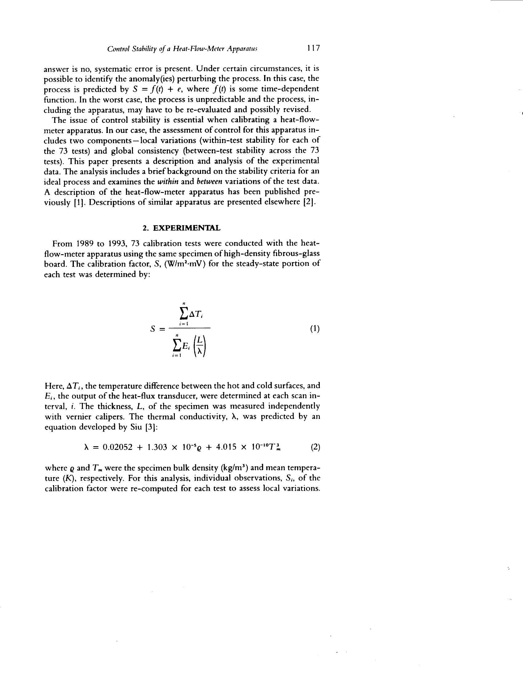
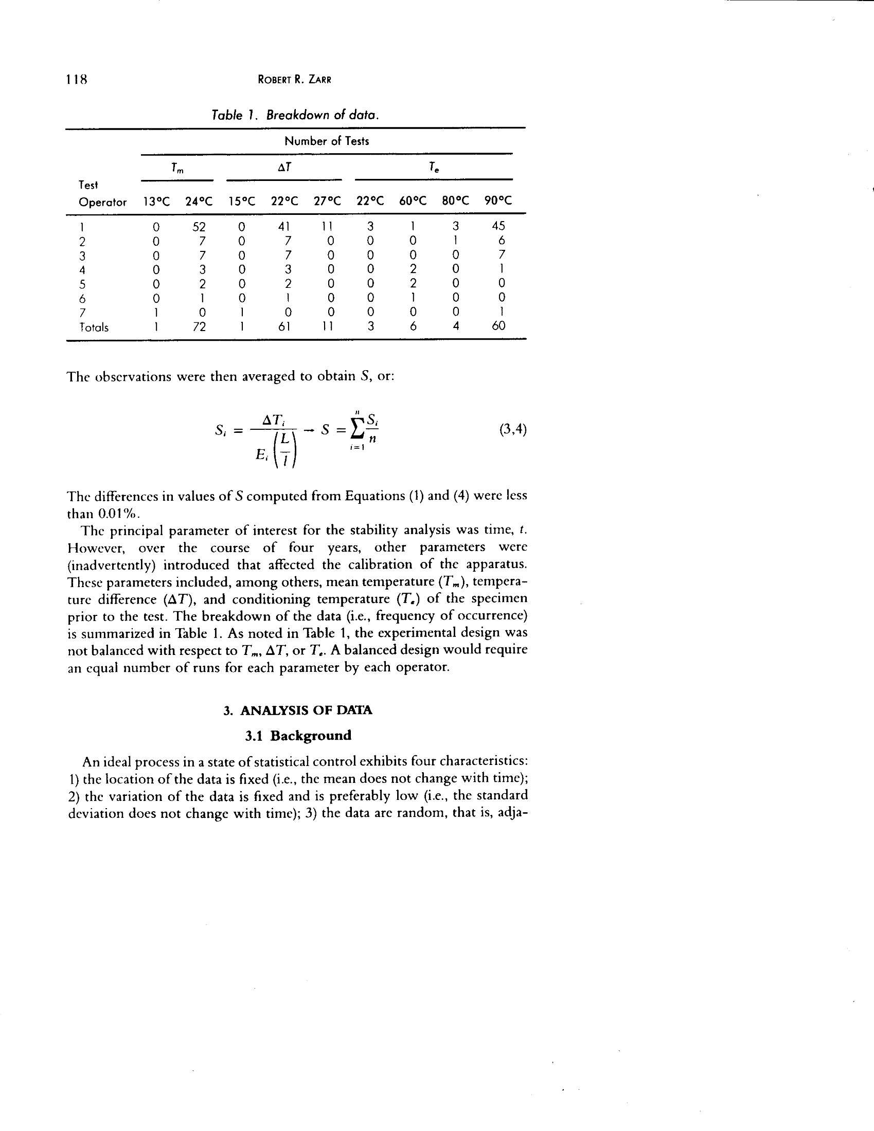
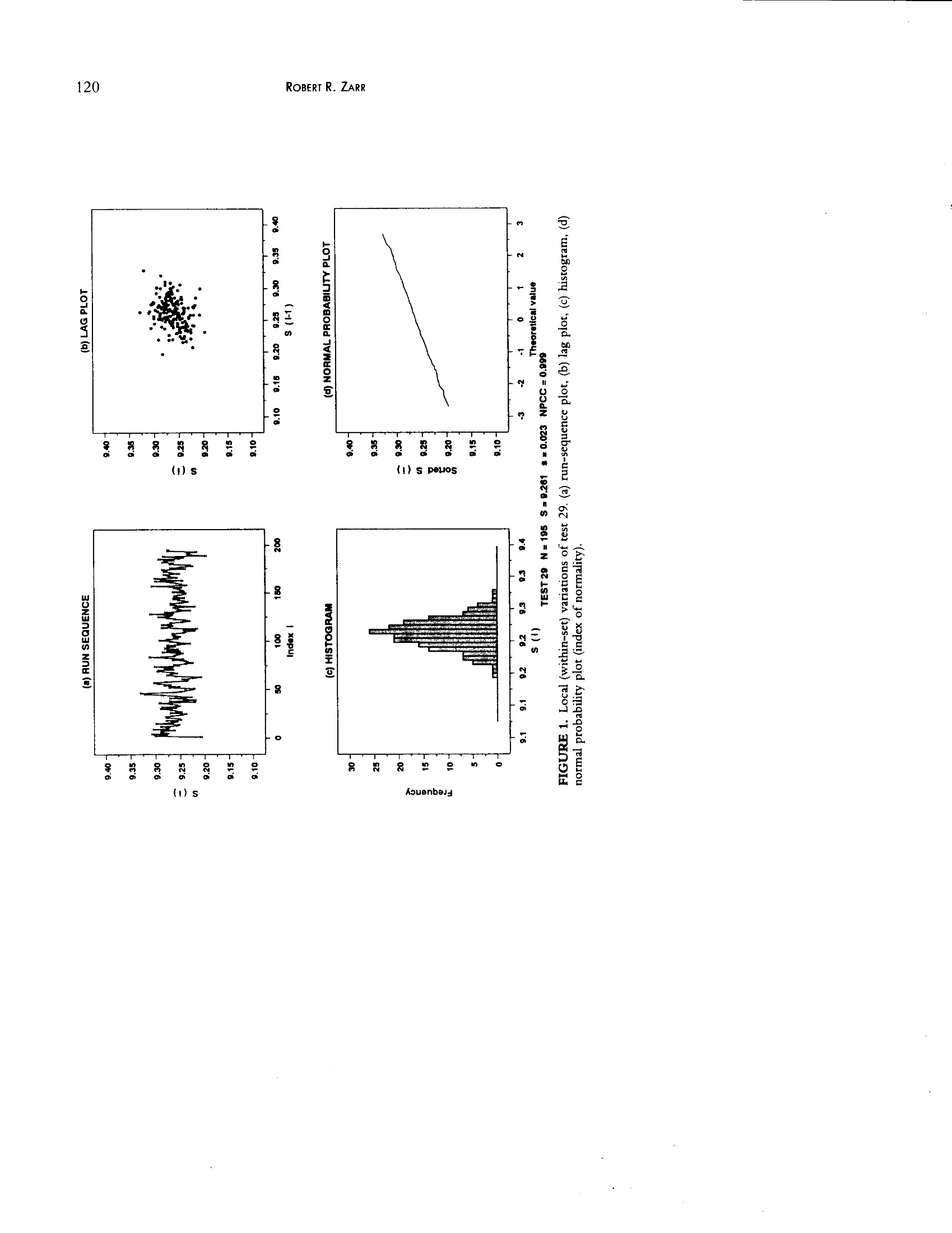
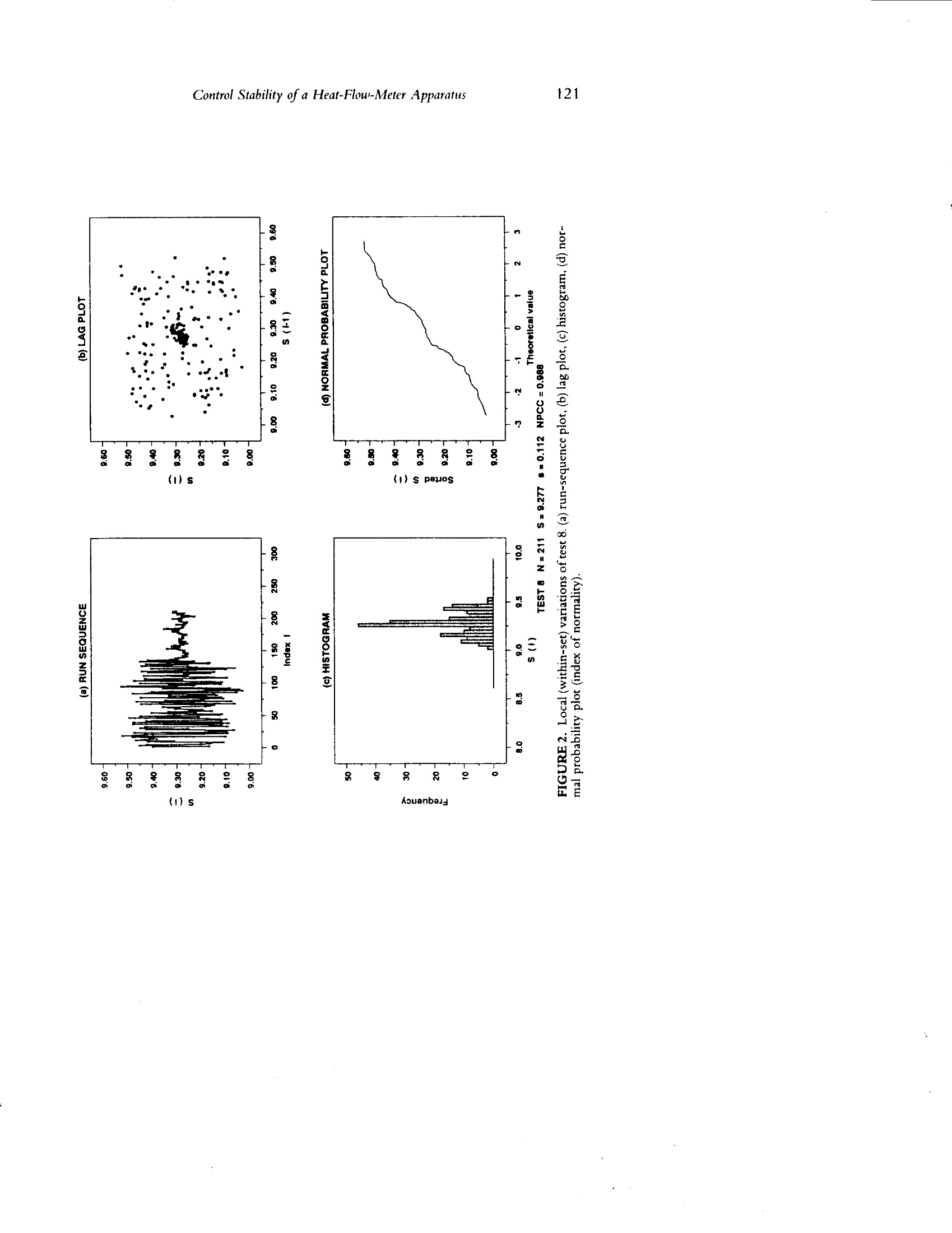
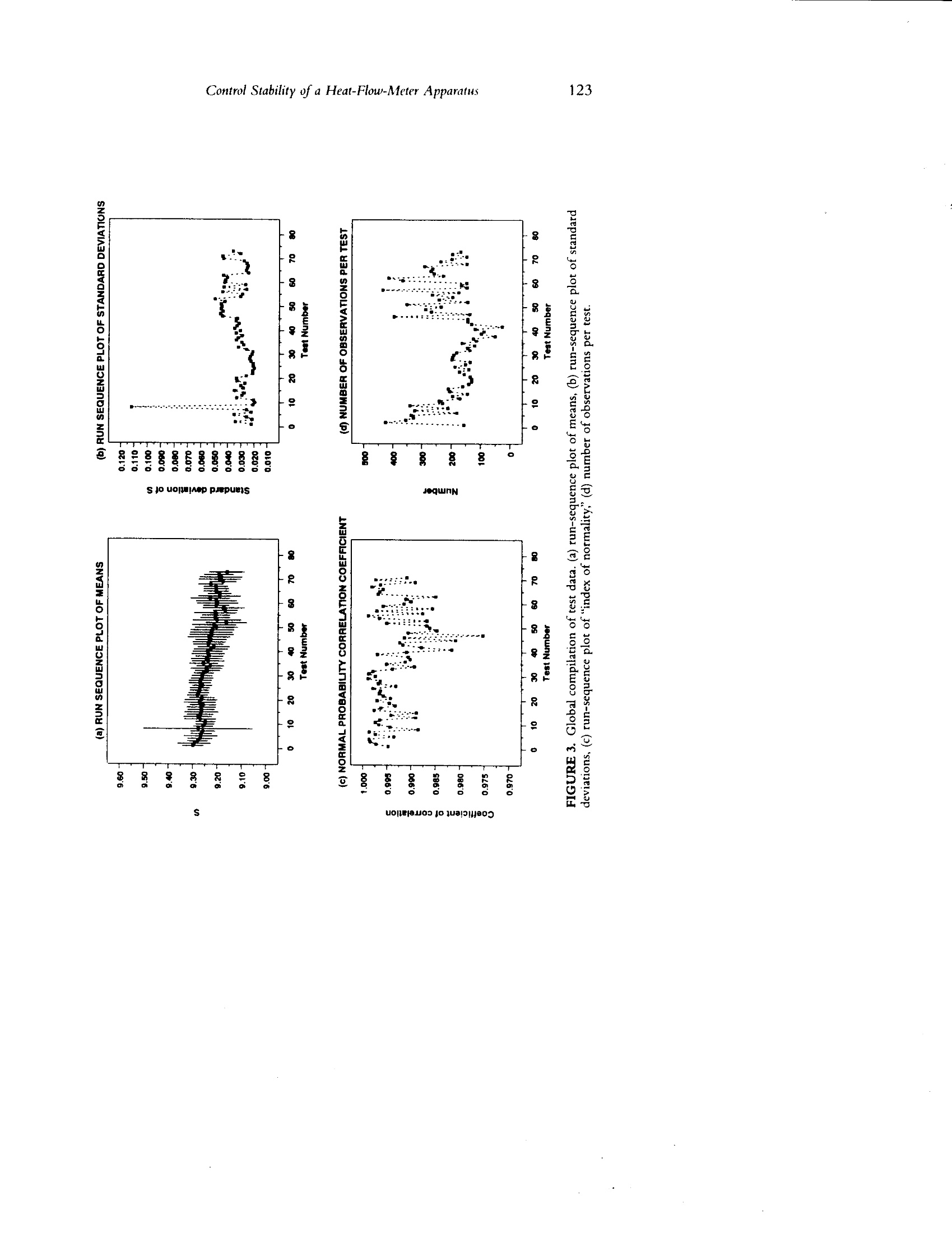
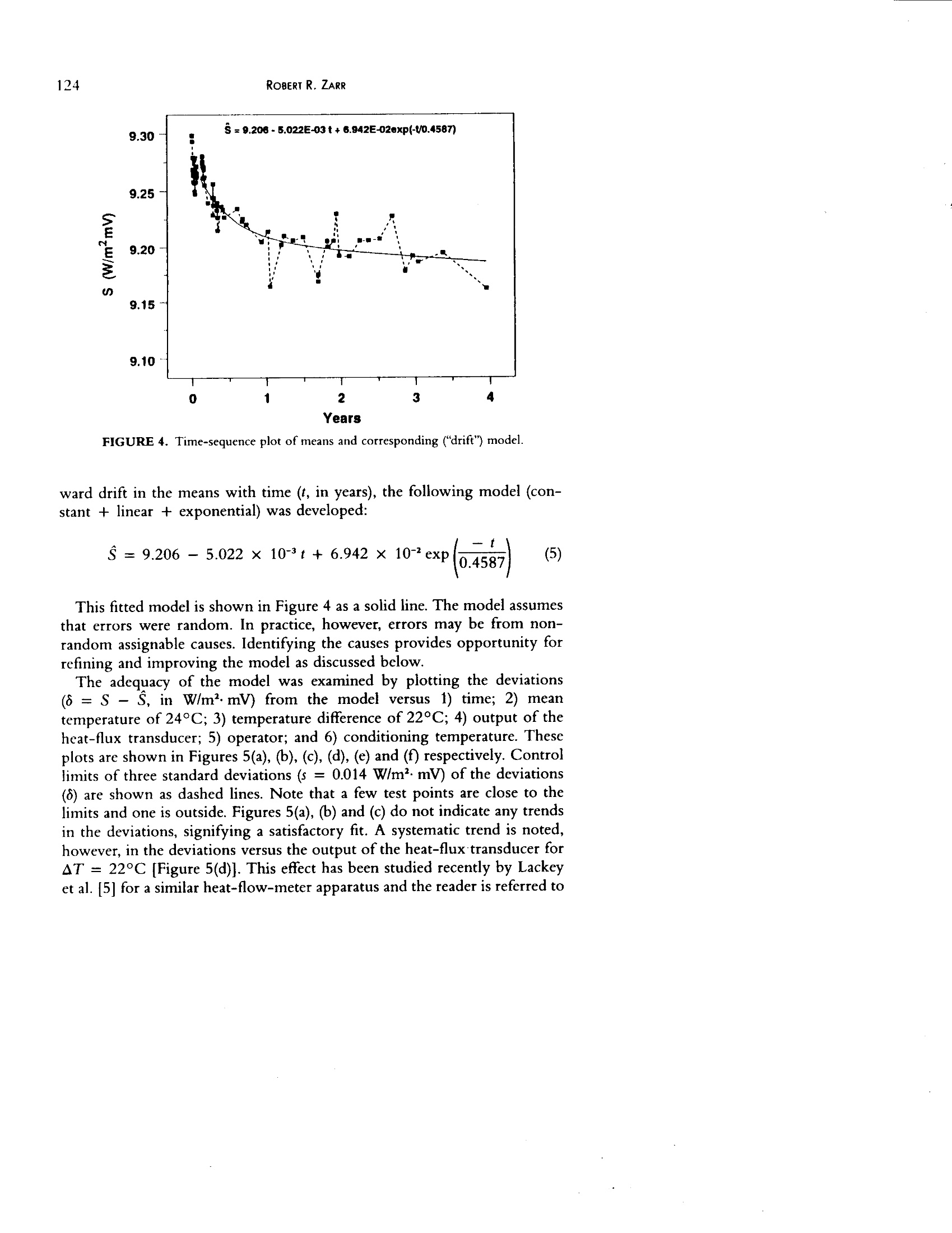
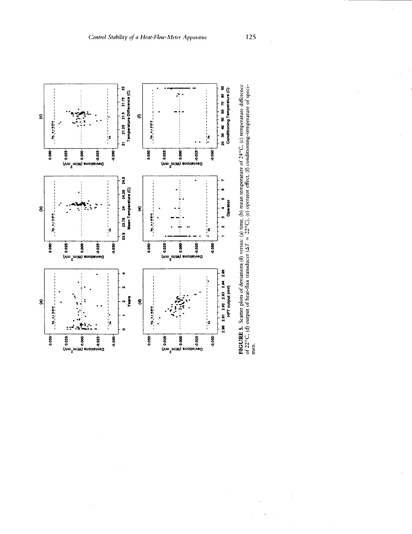
117Control Stability of a Heat-Flow-Meter Apparatus 118ROBERT R. ZARR Control Stability of aHeat-Flow-Meter Apparatus ROBERT R. ZARR Building and Fire Research Laboratory National Institute of Standards and Technology Gaithersburg, MD 20899 ABSTRACT: Calibration measurements of a commercial heat-flow-meter appara-tus are presented. The apparatus has been calibrated using the same specimen ofhigh-density fibrous-glass board over a period of four years, from 1989 to 1993.Seventy-three tests have been conducted, generally at ambient conditions of 24°Cwith a moderate temperature difference of either 15, 22 or 27°C across the specimen.Variations within a set of data for each test have been examined to verify underlyingassumptions of randomness, normal frequency distribution of errors, repeatability,and stability of the data. Variations between test data indicate a small drift, on theorder of one percent over four years, in the calibration factor of the apparatus. Amodel has been developed to describe the small drift with time. The analysis of varia-tions between test data has also identified intermittent shifts in the precision of thecalibration factor of the apparatus. 1. INTRODUCTION HE STABILITY PROBLEM can be re-stated as follows: is the heat-flow-meter apparatus "in statistical control"? That is, are the calibration factors(S)“in statistical control"? To ascertain the answer, a series ofcalibration testsare conducted and the resulting data analyzed for stability and consistency.If the answer is yes, the process is predicted by the equation: S = C + e,where C is a constant and e is random error. This equation assumes that theprocess is unbiased;in other words, systematic error is not present. If the ( This paper was o riginally presented at the American Society for Testing and Materials C-16Workshop on Measurement Errors and Methods of Calibration of Heat-Flow-Meter Apparatus at Wil- liamsburg, VA on April 9, 1994. ) ( Reprinted from J. THERMAL INSUL. AND BLDG.ENVS. Volume 18- October 1994 ) answer is no, systematic error is present. Under certain circumstances, it ispossible to identify the anomaly(ies) perturbing the process. In this case, theprocess is predicted by S =f(t) +e, where f(t) is some time-dependentfunction. In the worst case, the process is unpredictable and the process, in-cluding the apparatus, may have to be re-evaluated and possibly revised. The issue of control stability is essential when calibrating a heat-flow-meter apparatus. In our case, the assessment of control for this apparatus in-cludes two components-local variations (within-test stability for each ofthe 73 tests) and global consistency (between-test stability across the 73tests). This paper presents a description and analysis of the experimentaldata. The analysis includes a brief background on the stability criteria for anideal process and examines the within and between variations of the test data.A description of the heat-flow-meter apparatus has been published pre-viously ]. Descriptions of similar apparatus are presented elsewhere [2]. 2. EXPERIMENTAL From 1989 to 1993, 73 calibration tests were conducted with the heat-flow-meter apparatus using the same specimen of high-density fibrous-glassboard. The calibration factor, S, (W/m’mV) for the steady-state portion ofeach test was determined bv: Here, AT, the temperature difference between the hot and cold surfaces, andE, the output ofthe heat-flux transducer, were determined at each scan in-terval, i. The thickness, L, of the specimen was measured independentlywith vernier calipers. The thermal conductivity, 入, was predicted by anequation developed by Siu [3]: where g and Tm were the specimen bulk density (kg/m') and mean tempera-ture (K),respectively. For this analysis, individual observations, S, of thecalibration factor were re-computed for each test to assess local variations. Table 1. Breakdown of data. Number of Tests Tm AT Test Operator 13°CC 24°C 15°C 22°C 27°C 22°C 60°C 80°C 90°C 1 0 52 0 41 11 3 1 3 45 2 0 7 0 7 0 0 0 1 6 3 0 7 0 7 0 0 0 0 7 4 0 3 0 3 0 0 2 0 1 5 0 2 0 2 0 0 2 0 0 6 0 1 0 1 0 0 1 0 0 7 1 0 1 0 0 0 0 0 1 Totals 72 1 61 11 3 6 4 60 The observations were then averaged to obtain S, or: The differences in values of S computed from Equations (1) and (4) were lessthan 0.01%. The principal parameter of interest for the stability analysis was time, t.However, over the course of fouryears, other parameters Were(inadvertently) introduced that affected the calibration of the apparatus.These parameters included, among others, mean temperature (Tm), tempera-ture difference (AT), and conditioning temperature (T) of the specimenprior to the test. The breakdown of the data (i.e., frequency of occurrence)is summarized in Table 1. As noted in Table 1, the experimental design wasnot balanced with respect to Tm, AT, or T. A balanced design would requirean equal number of runs for each parameter by each operator. 3. ANALYSIS OF DATA 3.1 Background An ideal process in a state of statistical control exhibits four characteristics:1) the location of the data is fixed (i.e., the mean does not change with time);2) the variation of the data is fixed and is preferably low (i.e., the standarddeviation does not change with time); 3) the data are random, that is, adja- cent data“behave”independently of one another; and 4) the frequency distri-bution of the data is fixed (not changing with time) and, preferably,nor-mally distributed. The benefit of a process that is in a state of statisticalcontrol is predictability-the ability to predict where the process will be inthe future. As mentioned, the model that describes such an ideal process isS= C+ e. 3.2 Within-Set (Local) Variations The variations of observations (that is, calibration factor, S.) within eachset of test data were analyzed graphically to verify the underlying assump-tions of stability (fixed location and variation), randomness, and normality.A four-step method was applied: 1. a run-sequence plot (S., versus i)-checks for systematic and randomchanges 2. a lag plot (S. versus S;-)-checks for randomness 3. a histogram (of S.)-checks the frequency distribution 4. a normal probability plot (of S.)-checks the normality assumption This four-step analysis was executed for each of the 73 calibration tests.The analyses for two calibration tests, 29 and 8, are illustrated in Figures 1and 2 respectively, and summarized in Table 2. For most of the 73 data sets,the underlying assumptions were satisfied and thus the set of data deemed“in control Figure 1 shows the analysis for test 29 and illustrates an ideal"incontrol” process. Here, the location and variation [Figure 1(a)] are “fixed"(not changing with time). The lag plot [Figure 1(b)] has no discernablestructure and appears as a “bull's-eye.The histogram [Figure 1(c)] is bell-shaped; and the (normal) probability plot [Figure 1(d)] is linear. The test sta-tistic known as the normal probability correlation coefficient (NPCC) is dis-cussed elsewhere [4], but its graph is easy to interpret;if linear, then normal. The data from a few other tests were not normally distributed and, in fact,suggested an underlying bimodal mechanism. This mechanism is illustratedin the data of test 8 (Figure 2). Test 8 was the only test that failed to satisfy Table 2. Summary of within-set assumption for tests 29 and 8. Criteria 29 8 1. Fixed location? Yes Yes 2. Fixed variation? Yes No 3. Randomness assumption? Yes No 4. Normality assumption? Yes No FIGURE 1. Local (within-set) variations of test 29. (a) run-sequence plot, (b) lag plot,(c) histogram,(d)normal probability plot (index of normality). FIGURE 2. Local (within-set) variations of test 8. (a) run-sequence plot, (b) lag plor, (c) histogram,(d) nor-mal probability plot (index of normality). the assumption of fixed variation [Figure 2(a)]. After further investigation,the source of variation was traced to the output of the heat-flux transducer.As noted in Figure 2a, the data falls into two groups. Although the meansfor both groups of observations were essentially the same, the standard devi-ations were different by a factor of about 8. This behavior was not sympto-matic of the transducer itself, but instead, of some external electrical con-tamination. At present, the external contamination has not been identified. 3.3 Between-Set (Global) Consistency The same questions concerning changes in variation, location, as well asnormality were examined globally by checking consistency between the 73sets of test data. A graphical compilation of the 73 tests is illustrated inFigure 3. Figure 3(a) shows a run sequence of means where S is plottedagainst test number (1 to 73, inclusive). Included with each point are errorbars of twice the standard deviation of each mean. Three characteristics inthe data were observed: 1) a downward drift of about one percent in themeans; 2) a large variability for test 8 (discussed above); and, 3) small(neglecting test 8) changes in the standard deviations. As noted in the run-sequence plot of standard deviations [Figure 3(b)], the changes were ac-tually small intermittent shifts. The source of these shifts was traced tochanges in the output of the heat-flux transducer as discussed above. The in-dex of normality [Figure 3(c)] indicated that about two-thirds of the testdata were normally distributed (coefficients≈ 1). Further analysis is re-quired to explain non-normal data sets. The number of observations per testis shown in Figure 3(d). 4. MODEL FOR GLOBAL DATA A time-sequence plot of the means (S versus t) is shown in Figure 4. Theinitial time, t=0, denotes the apparatus’s return from the manufacturerafter renovation, which included installation of: 1) a new heat-flux transduc-er; 2) new digital temperature controllers; and 3) new type-K* thermo-couples [1]. Since the apparatus was essentially new, most of the data wascollected within the first half-year to verify the operation of the apparatus.As time progressed, the calibration tests were conducted at greater time in-tervals. If the apparatus was “in control"for all 73 tests, then the appropriatemodel would be: S=C +e. From Figures 3(a) and 4, it is clear this wasnot the case. Instead, there was a downward drift. To account for the down- ( *Nickel and 1 0 p ercent chromium versus nickel a nd 5 p ercent aluminum a n d silicon. ) oo2ooEooE令:2EoooaE2o Control Stability ofa Heat-Flow-Meter Apparatus FIGURE 4. Time-sequence plot of means and corresponding ("drift") model. ward drift in the means with time (t,in years), the following model (con-stant + linear+ exponential) was developed: This fitted model is shown in Figure 4 as a solid line. The model assumesthat errors were random. In practice, however, errors may be from non-random assignable causes. Identifying the causes provides opportunity forrefining and improving the model as discussed below. The adequacy of the model was examined by plotting the deviations(8=S- S, in W/m’ mV) from the model versus11) time; 2) meantemperature of 24°C; 3) temperature difference of 22°C; 4) output of theheat-flux transducer; 5) operator; and 6) conditioning temperature. Theseplots are shown in Figures 5(a), (b), (c), (d), (e) and (f) respectively. Controllimits of three standard deviations (s = 0.014 W/m’ mV) of the deviations() are shown as dashed lines. Note that a few test points are close to thelimits and one is outside. Figures 5(a), (b) and (c) do not indicate any trendsin the deviations, signifying a satisfactory fit. A systematic trend is noted,however, in the deviations versus the output of the heat-fluxtransducer forAT= 22°C [Figure 5(d)]. This effect has been studied recently by Lackeyet al. [5] for a similar heat-flow-meter apparatus and the reader is referred to aoEuocaooo that paper for further details. Other systematic trends are noted in Figures5(e) and (f), particularly at a conditioning temperature of 22°C. In order toconclude which of these parameters affected the calibration, confoundingeffects must be eliminated by conducting a balanced-design experiment. 5. SUMMARY Over a period of four years, 73 calibration tests of a heat-flow-meter ap-paratus were conducted with a single specimen of fibrous-glass board. Mosttests were conducted at 24°C with either a temperature difference of 15, 22or 27°C. An analysis of local variations of the test observations indicatedthat most of the sets of data were in a state of statistical control. There were,however, small intermittent shifts in the repeatability (within-laboratoryprecision) of the calibration factor due to changes in the output of the ap-paratus's heat-flux transducer. A global check of the test data revealed asmall downward drift, on the order of one percent, in the calibration factorover the four-year period. A model of the form: S = ao + at + az exp(t/as)was fit to the data to account for the drift with time (t). An analysis of thedeviations from the model indicated further improvement in the modelcould be obtained by considering other factors, such as the output of theheat-flux transducer, operator, and pre-conditioning temperature of thespecimen. 6. ACKNOWLEDGEMENTS The author appreciates discussions with Dr. Jim Filliben of the StatisticalEngineering Division of NIST. The author also acknowledges the followingstudents who assisted with the data collection and preparation of the manu-script: John Judge, Kevin Simmons, Mike Price, Dan Shapiro, ChrisSaunders, Ken Kramp, and Holly Chandler. REFERENCES 1. Zarr,R. R. and B. A. Licitra. 1991.“Calibration at 24°C of a Heat-Flow-MeterApparatus Having 610 mm Square Plates, NISTIR 4539 (May). 2.ASTM. 1991. “Standard Test Method for Steady-State Heat Flux Measurementsand Thermal Transmission Properties by Means of the Heat Flow Meter Appara-tus,ASTM C518-91, Annual Book of ASTM Standards, American Society for Test-ing and Materials, Philadelphia. 3. SSiu, M. C. I. 1980.“Fibrous Glass Board as a Standard Reference Material forThermal Resistance Measurement Systems,ASTM STP 718, Thermal Insulation Performance, D. L. McElroy and R. P. Tye, eds., Philadelphia, American Society forTesting and Materials, pp. 343-360. 4. Flilliben,J. J. 1975.“The Probability Plot Correlation Coefficient Test for Nor-mality,” Technometrics, 17:111-117, (February). 5.Lackey, et al. 1994.“Calibration of the Heat Flow Meter Apparatuses at theNRCC," Journal of Thermal Insulation (this publication).
确定

还剩10页未读,是否继续阅读?

产品配置单
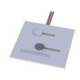
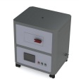
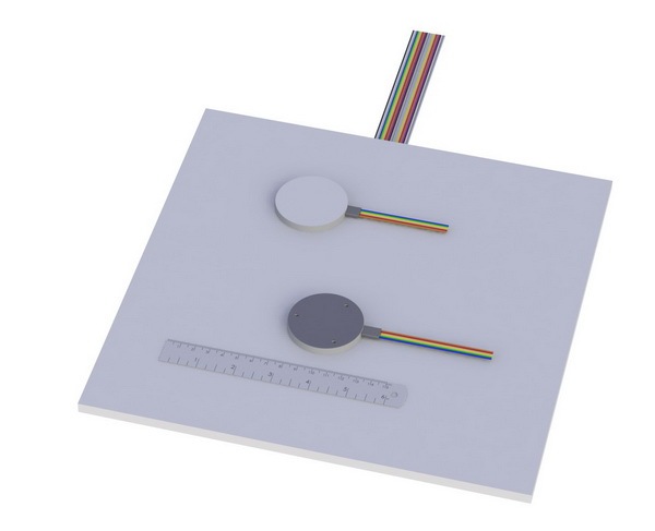
上海依阳实业有限公司为您提供《热流计校准装置的稳定性控制》,该方案主要用于其他中检测,参考标准--,《热流计校准装置的稳定性控制》用到的仪器有高灵敏度热阻式热流计、稳态护热板法导热系数测定仪
推荐专场
相关方案
更多
该厂商其他方案
更多